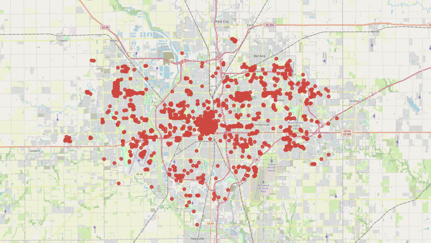
OpenStreetMap (OSM) data is a “treasure trove” hiding in plain sight for any journalistic mapping project. Here, we present how one can retrieve and process OpenStreetMap data using Python or QGIS.
Mapping can offer significant advantages to a journalistic piece. It can depict an issue in a more “well-rounded” way, serve as a starting point for further investigation, or even as a stand alone piece, with a map that is useful to the public. In such an endeavor, OpenStreetMap (OSM) data is a “treasure trove” in plain sight. It is a collaborative mapping project that offers its data freely to everyone (under the Open Database License), and to which anyone can contribute.
However, this data is presented in the same way as on other similar maps. So the “key” to analyzing it is to access it through specialized software or programmatically. Below, we present two approaches we used, along with examples, to map features in cities and countries around the world.

The data structure
Before moving on to the examples, we should first explain the structure of the data as it is organized within OpenStreetMap (OSM). The most fundamental building block of the conceptual data model that OSM applies is its “elements” — something like the building blocks that construct the world. There are three types of elements:
- Nodes, which define points: a restaurant, a pharmacy, a bench, etc.
- Ways (lines), which can either define a linear feature (e.g., a railway line) or enclose the boundaries of an area, creating a polygon (for example, a country’s borders, or the boundaries of an airport and its facilities).
- Relations, which define the interaction between other elements (e.g., a bus route and the avenue it passes through).
In our analysis, we searched only for nodes and ways, in order to locate specific features within the areas of interest. Specifically, as an illustrative example, below we will retrieve data — in two different ways — on parking facilities in Kansas. The same approach can be utilised though in any other part of the world.
Checking features on OpenStreetMap
Before proceeding to data retrieval, it makes sense to check the features via a browser on OSM. For example, suppose we are interested in data on Athens, Greece:
- We open OSM in the browser and, in the search bar, type “Athens.” The map zooms in on the capital of Greece, and a pin appears at its center.
- We zoom in and right-click on the city center, then select “Query Features.” A left-hand side menu then opens: there, under “Enclosing Features,” we can see that “Administrative Boundary (Level 7) Municipality of Athens” is included. Selecting it, we see the full administrative boundary element of the Municipality of Athens, and under “Tags” the name of the city as it appears in the system: “Municipality of Athens.”
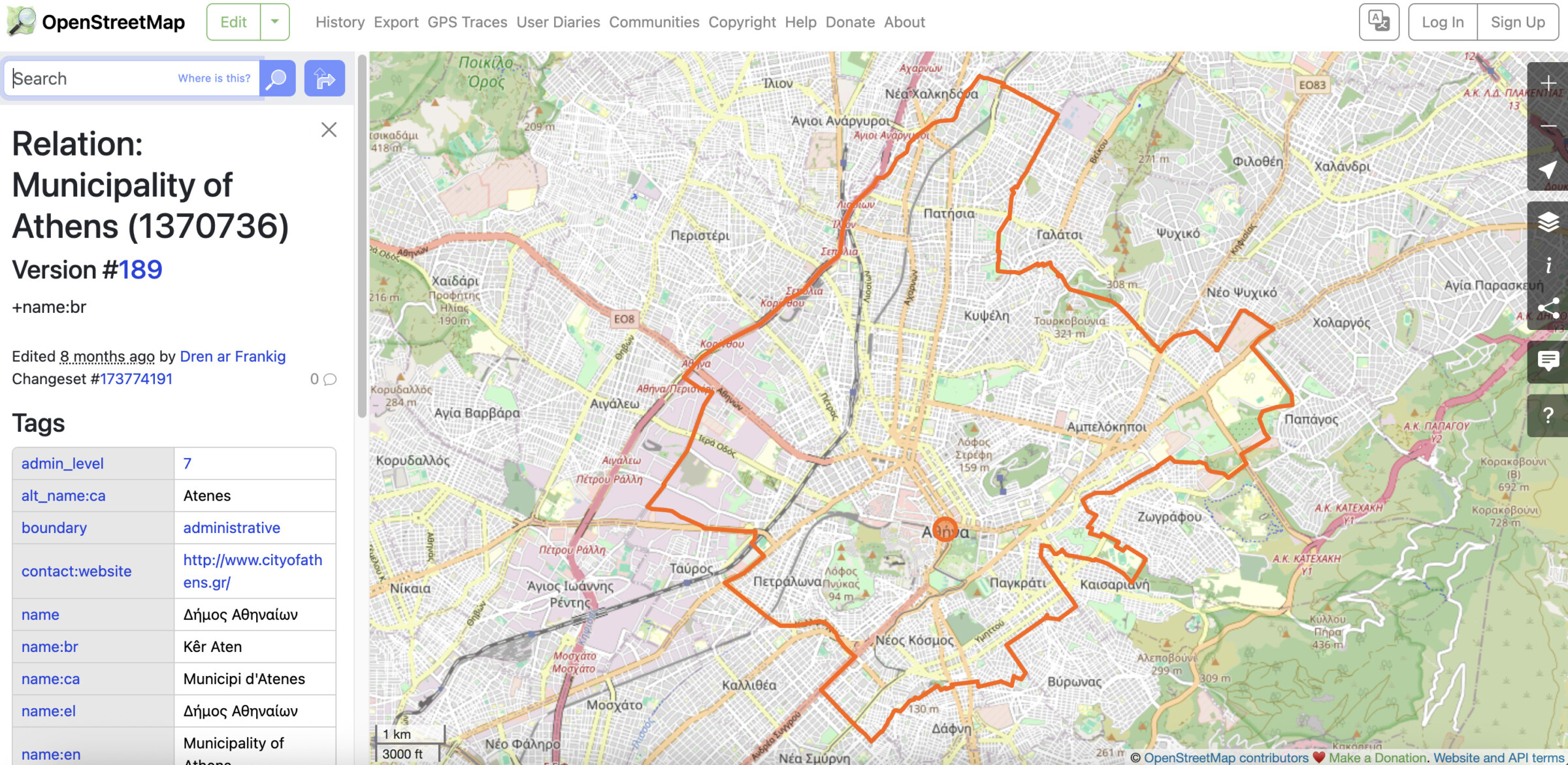
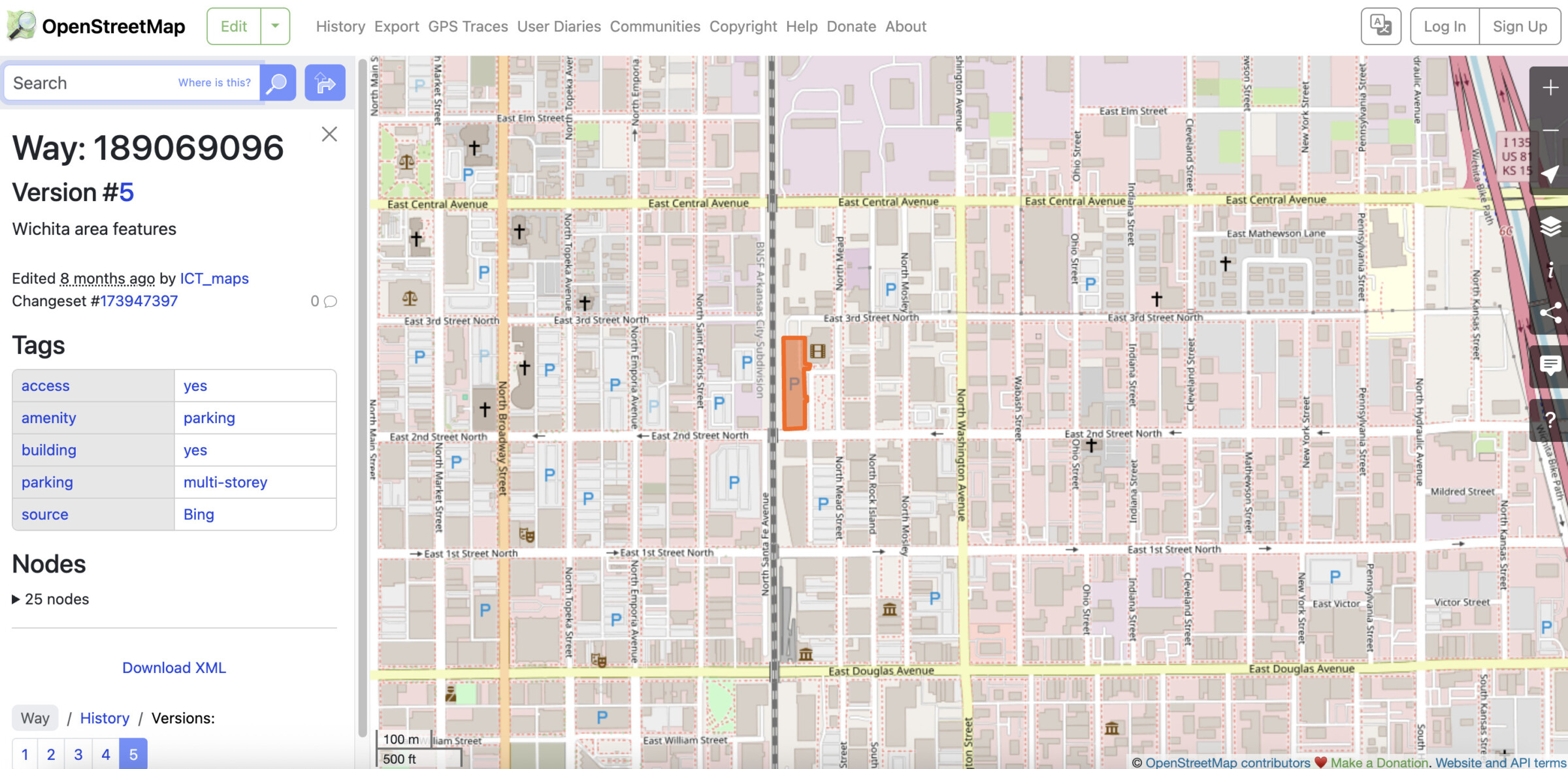
Similarly, to identify the correct term for the features we want to search for, we consult the “Tags.” These consist of two parts: a primary one (e.g., “amenity”) and a secondary one (e.g., “parking”). Just as with the name of Athens, for each category of features we wish to map, we must identify the correct terminology using the same process.
Approach 1: Retrieving data with Python
In the first — and admittedly more complex — method, we use a script, written in the Python programming language, to download the full set of features for the area of interest, and then identify, within that full set, those that are relevant to the analysis.
In the first step, we define the area of interest. It must be defined in English and in exactly the same way as it appears within the OSM maps — like “Municipality of Athens” or “Wichita” for Wichita, Kansas, which we are using in our example.
The data is downloaded using the quackosm library from a server operated by Geofabrik, a German company that provides free daily extracts of OpenStreetMap data.
In the next step, the code retrieves the features that have the parameters we selected (in our example, “amenity” + “parking”) within the area of interest, and gathers them into a dataframe with geographic coordinates.
Code that maps the parking spaces in Wichita, Kansas
!pip install quackosm folium geopandas -q
import quackosm as qosm
import geopandas as gpd
from shapely.ops import unary_union
import folium
from IPython.display import display
import pandas as pd
import colorsys


# ─── CHANGE ONLY THIS BLOCK ───────────────────────────────────────────────────

PLACES = [
    "Wichita",
]

TAGS = {
    "amenity": ["parking" ]
}

DISPLAY_COLS = ["name", "amenity"]

# ──────────────────────────────────────────────────────────────────────────────

geometries = [qosm.geocode_to_geometry(p) for p in PLACES]
geometry_filter = unary_union(geometries)
gdf = qosm.convert_geometry_to_geodataframe(
    geometry_filter=geometry_filter,
    tags_filter=TAGS,
    osm_extract_source="Geofabrik",
    keep_all_tags=True,
    explode_tags=False,
    verbosity_mode="transient",
)
gdf["name"]    = gdf["tags"].apply(lambda t: t.get("name")    if isinstance(t, dict) else None)
gdf["amenity"] = gdf["tags"].apply(lambda t: t.get("amenity") if isinstance(t, dict) else None)
cols_to_show = [c for c in DISPLAY_COLS if c in gdf.columns]


if gdf.empty:
    print("No features found.")
else:
    TAG_COLS = [c for c in gdf.columns if c not in ("geometry", "tags", "name")]

    def get_feature_label(row):
        tags = row.get("tags")
        if not isinstance(tags, dict):
            return "other"
        for key in TAGS:
            val = tags.get(key)
            if val and pd.notna(val):
                return f"{key}: {val}"
        for key, val in tags.items():
            if val and pd.notna(val):
                return f"{key}: {val}"
        return "other"

    gdf["_label"] = gdf.apply(get_feature_label, axis=1)
    unique_labels = sorted(gdf["_label"].unique())

    def make_palette(n):
        palette = {}
        for i, label in enumerate(unique_labels):
            if label == "other":
                palette[label] = "#72D61A"
            else:
                hue = i / max(n, 1)
                r, g, b = colorsys.hsv_to_rgb(hue, 0.75, 0.88)
                palette[label] = "#{:02x}{:02x}{:02x}".format(
                    int(r * 255), int(g * 255), int(b * 255)
                )
        return palette

    palette = make_palette(len(unique_labels))

    bounds = gdf.total_bounds
    center_lat = (bounds[1] + bounds[3]) / 2
    center_lon = (bounds[0] + bounds[2]) / 2

    m = folium.Map(
        location=[center_lat, center_lon],
        zoom_start=12,
        tiles="CartoDB positron"
    )
    folium.TileLayer("OpenStreetMap", name="OpenStreetMap").add_to(m)

    for _, row in gdf.iterrows():
        name = row.get("name") or "Unnamed"
        geom = row.geometry
        point = geom if geom.geom_type == "Point" else geom.centroid
        label = row["_label"]
        color = palette[label]

        tags = row.get("tags") or {}
        popup_fields = [f"<b>{name}</b>"] + [
            f"{k}: {v}" for k, v in tags.items() if v and pd.notna(v)
        ]
        popup_html = "<br>".join(popup_fields)

        folium.CircleMarker(
            location=[point.y, point.x],
            radius=6,
            color=color,
            fill=True,
            fill_color=color,
            fill_opacity=0.85,
            tooltip=f"{name} ({label})",
            popup=folium.Popup(popup_html, max_width=280),
        ).add_to(m)

    legend_items = "".join(
        f'<div style="display:flex;align-items:center;margin-bottom:5px">'
        f'<div style="width:14px;height:14px;border-radius:50%;background:{color};'
        f'margin-right:8px;flex-shrink:0"></div>'
        f'<span style="font-size:12px">{label}</span></div>'
        for label, color in sorted(palette.items())
    )
    legend_html = f"""
        <div style="
            position: fixed; bottom: 40px; left: 40px; z-index: 1000;
            background: white; padding: 12px 16px; border-radius: 8px;
            box-shadow: 0 2px 8px rgba(0,0,0,0.2); max-height: 320px;
            overflow-y: auto; font-family: sans-serif;
        ">
        <div style="font-weight:bold;margin-bottom:8px;font-size:13px">Feature types</div>
        {legend_items}
        </div>
    """
    m.get_root().html.add_child(folium.Element(legend_html))
    folium.LayerControl().add_to(m)
    m.fit_bounds([[bounds[1], bounds[0]], [bounds[3], bounds[2]]])
    display(m)

A dataset is always useful, but it’s even more practical if it is visualized on a map — especially an interactive one. So, in the final step of our code, we use the folium library to map the features we have gathered.
We dynamically create a color palette to visually differentiate the various features we may have collected. The differentiation is based on the secondary attribute. So, for example, if there are more than two “amenities” (“parking,” “place of worship”), each will receive its own distinct color. Also, to make the visualization of the features more uniform, we convert the polygons into points by identifying their centroid — that is, their central point.
This approach is more complex, given that it also requires basic knowledge of Python, but it can prove useful if one does not want to “burden” their computer with additional software. After all, the same code can run in the cloud, using a Google Colab Notebook.

Approach 2: QGIS and a small plug-in
The easiest method for locating features without getting into code development is to use QGIS, the free, open-source geospatial analysis software with which one can create and edit geospatial data.
For installation and a broader guide on how to use QGIS, find more information here.
To download OSM data into your project within QGIS, you must have installed the “QuickOSM” plug-in. To do this, simply go to the options at the top left of your screen within QGIS, select “Plugins” and then “Manage and Install Plugins.” Then, search for “QuickOSM” and install it in QGIS. Once you have installed it successfully, you will have the green search icon above the “Layers” panel.
An essential step for working with this data is to first open an OSM map layer within QGIS, so that the features are visible on a map. To do this, follow this path: Layer > Add Layer > Add XYZ Layer.

In the final step, from the “Custom” menu, select OpenStreetMap and click “Add” at the bottom right of the window.

Upon opening QuickOSM (the green search icon), you will be presented with a list of preset queries you can run. However, to gather the list of objects you want, for the area you want, click “Quick query” (on the left).

There, you will need to fill in the features you want to find, following the same logic we used in the Python approach. So, in this case, to locate all parking facilities in the city of Wichita, Kansas, we will enter “amenity” in the key field and “parking” in the value field. Then there is the area menu. Several different options are offered here:

- “In”: we locate all features that lie within a geographic area — in this case, within the administrative boundaries of the city of Wichita, which we have seen exists in OSM as “Wichita.”
- “Around”: finds the features that lie within a specified radius of a geographic feature.
- “Canvas extent”: with this option, we do not specify a particular area for locating features, as everything visible on the map within your environment in QGIS is downloaded.
- “Layer extent”: with this approach, all features located within the geographic boundaries of an already existing layer are downloaded. For example, you have a polygon layer containing the boundaries of a Natura area. With this option, you will find all the features within it.
- “Non spatial”: all selected features are downloaded without any geographic boundary specification.
By following these steps, we have therefore gathered all the parking facilities within the administrative boundaries of the city of Wichita, Kansas, as recorded in OSM.

If we want to go one step further, for a uniform visualization of the features, we identify their centroid, so that both polygons and lines have the same form on the map. To calculate this, the process is: Vector > Geometry Tools > Centroids. Then, we select the layer we wish to process and click “Run.” Thus you will have a point for each feature, and the features will be visible in all the levels of zoom of the map.