How far away is the nearest school? We used secondary schools across rural Greece as a case study to map distances to an essential service and demonstrate how isodistances can be calculated and visualized on a map.
Part of the vicious cycle in addressing the demographic problem in Greece is the relationship between population decline in rural regions and the simultaneous withdrawal of services from those areas, since fewer residents cannot justify the presence of many shops and public services. Thus, the problem of distance often comes to the forefront (e.g. the closure of ELTA post office branches, the closure of school units, the availability of health services), as a citizen in some remote settlement often cannot easily access basic services.
To further analyze this problem — one that is not exclusively Greek — we created this practical article, as a resource for calculating isodistances, i.e. “zones” of distance from services. In this case, we used as an example the secondary level school (Gymnasium and Lyceum) units in Greece, excluding the areas of Attica and Thessaloniki, where the main cities are located.
Code and a free tool
To extract the isodistances we used the API of the free openrouteservice, which was created by the Heidelberg Institute for Geoinformation Technology (HeiGIT), which in turn uses OpenStreetMap’s geospatial data to calculate the isodistance zones. The school unit data comes from the Panhellenic School Network (PSD), the national network and internet service provider of the Greek Ministry of Education and Religious Affairs, which connects and supports more than 16,000 units.
We downloaded the data of active school units from the PSD website, by region, in .xlsx format, and merged them into a single dataset (available here). The dataset includes information on 15,097 active school and administrative units across the country. Attica and Thessaloniki were excluded from this analysis and visualization due to the large number of school units and their relatively short distance from each other. As a result, 2,296 school units are included in the map below.
Retrieving and processing OpenStreetMap data
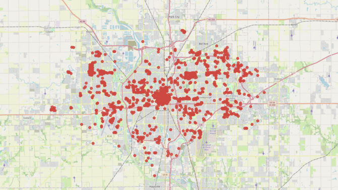
OpenStreetMap (OSM) data is a “treasure trove” hiding in plain sight for any journalistic mapping project. We present how one can retrieve and process OpenStreetMap data using Python or QGIS.
An isodistance zone is an area extending from a geographic point, within which the distance from said point does not exceed a certain number of kilometers/meters. For example, in the map below, dark blue shows the area within which the iconic Notre-Dame de Paris (the red marker) is less than one kilometer away, while light teal shows the zone within which it is less than two kilometers away. This calculation is not made as if it were the radius of a circle, in a straight line, but takes into account the road network of the area, in order to determine how a pedestrian or a vehicle would actually get there.

Due to the limit that openrouteservice applies to isodistance processing (500 per day), we chose to proceed with the calculation of isodistances only for middle schools and high schools. Since the number of school units is again above the limit (more than 2,000), the code we wrote includes provisions for the calculation to be carried out in separate batches.
Code for calculating the isodistances from each school
# ── 0. Install
!pip install -q geopandas folium shapely openrouteservice pyogrio

# ── 1. Imports
import time
import pickle
from pathlib import Path
import pandas as pd
import geopandas as gpd
import folium
import openrouteservice as ors
from shapely.geometry import shape
from openrouteservice.exceptions import ApiError


# ── 2. Configuration

RADII_KM = [5, 10, 25, 50]
COLORS = {
    5: "#2166ac",
    10: "#74add1",
    25: "#fdae61",
    50: "#d73027",
}

CHECKPOINT = Path("/content/isodistances_raw.pkl")
ERRORS_CSV = "/content/isodistances_errors.csv"
OUTPUT_GPKG = "/content/isodistances.gpkg"
OUTPUT_HTML = "/content/isodistances_road.html"

# Safe rate for the standard isochrone limit
SLEEP_SECONDS = 3.2
MAX_RETRIES = 3


# ── 3. Prepare locations
nip = df_test.copy()

nip["Γεωγραφικό Πλάτος"] = pd.to_numeric(
    nip["Γεωγραφικό Πλάτος"],
    errors="coerce",
)

nip["Γεωγραφικό Μήκος"] = pd.to_numeric(
    nip["Γεωγραφικό Μήκος"],
    errors="coerce",
)

nip = nip.dropna(
    subset=[
        "Κωδικός ΜΜ",
        "Ονομασία",
        "Γεωγραφικό Πλάτος",
        "Γεωγραφικό Μήκος",
    ]
).copy()

nip = nip[
    nip["Γεωγραφικό Πλάτος"].between(-90, 90)
    & nip["Γεωγραφικό Μήκος"].between(-180, 180)
].copy()

origins_gdf = gpd.GeoDataFrame(
    nip,
    geometry=gpd.points_from_xy(
        nip["Γεωγραφικό Μήκος"],
        nip["Γεωγραφικό Πλάτος"],
    ),
    crs="EPSG:4326",
)

print(f"✓ Valid locations for calculation: {len(origins_gdf)}")


# ── 4. Create ORS client
client = ors.Client(
    key=ORS_KEY.strip(),
    base_url="https://api.heigit.org/openrouteservice",
)


# ── 5. Load existing checkpoint, if available
if CHECKPOINT.exists():
    with CHECKPOINT.open("rb") as f:
        results = pickle.load(f)
    print(f"✓ Loaded checkpoint with {len(results)} completed origins")
else:
    results = {}

errors = []


# ── 6. Calculate isodistances for all df_test locations
for position, (_, row) in enumerate(origins_gdf.iterrows(), start=1):
    mm_id = row["Κωδικός ΜΜ"]

    # Skip locations already successfully obtained in a prior run.
    if mm_id in results:
        continue

    lat = float(row["Γεωγραφικό Πλάτος"])
    lon = float(row["Γεωγραφικό Μήκος"])

    try:
        for attempt in range(1, MAX_RETRIES + 1):
            try:
                response = client.isochrones(
                    locations=[[lon, lat]],  # ORS coordinate order: [lon, lat]
                    profile="driving-car",
                    range_type="distance",
                    range=[radius * 1000 for radius in RADII_KM],
                )
                break

            except ApiError as e:
                error_text = str(e)

                # Retry only rate limiting, with increasing pauses.
                if "429" in error_text and attempt < MAX_RETRIES:
                    wait_seconds = 30 * attempt
                    print(
                        f"Rate limit at {position}/{len(origins_gdf)}. "
                        f"Waiting {wait_seconds}s; retry {attempt + 1}/{MAX_RETRIES}."
                    )
                    time.sleep(wait_seconds)
                    continue

                raise

        results[mm_id] = {
            "name": row["Ονομασία"],
            "lat": lat,
            "lon": lon,
            "features": response["features"],
        }

        print(
            f"✓ {position}/{len(origins_gdf)} "
            f"| {mm_id} | total cached: {len(results)}"
        )

    except Exception as e:
        errors.append({
            "position": position,
            "Κωδικός ΜΜ": mm_id,
            "Ονομασία": row["Ονομασία"],
            "lat": lat,
            "lon": lon,
            "error": str(e),
        })

        print(f"✗ {position}/{len(origins_gdf)} | {mm_id}: {e}")

        # A 403 is an access/key/host-side problem: persist results and stop.
        # Re-run later; cached locations will be skipped.
        if "403" in str(e):
            print("Stopping after 403; checkpoint has been saved.")
            break

    finally:
        with CHECKPOINT.open("wb") as f:
            pickle.dump(results, f)

        pd.DataFrame(errors).to_csv(ERRORS_CSV, index=False)

        time.sleep(SLEEP_SECONDS)

print(f"\nFinished or paused.")
print(f"Completed origins: {len(results)}")
print(f"Errors recorded: {len(errors)}")One key problem we faced when trying to calculate the isodistances with openrouteservice was maritime connections. HeiGIT’s service includes ferry routes in its calculation as if they were a road connection. This obviously had to be corrected. So, in a second stage, after we had already calculated the isodistances for the island school units, we restricted the polygons of the kilometer zones to within their coastline boundaries, with the exception of the two Greek islands that have a land connection: Evia and Lefkada.
Creation of an interactive map
# ─ 0. Imports
import pickle
from pathlib import Path
from collections import defaultdict
import geopandas as gpd
import folium
from shapely.geometry import Point, box, shape, mapping
from shapely.ops import unary_union
from folium.plugins import MarkerCluster


# ── 1. Configuration
CHECKPOINT = Path("/content/isodistances_raw.pkl")

COLORS = {
    5: "#2166ac",
    10: "#74add1",
    25: "#fdae61",
    50: "#d73027",
}

OUTPUT_MAP = "/content/isodistances_strict_coastline.html"


# ── 2. Load isodistance results
with CHECKPOINT.open("rb") as f:
    results = pickle.load(f)

if not results:
    raise ValueError("Checkpoint contains no ORS results.")

print(f"✓ Loaded {len(results)} origins from checkpoint")


# ── 3. Load high-resolution Natural Earth land polygons
print("Loading high-resolution land polygons...")

world_land = gpd.read_file(
    "https://naciscdn.org/naturalearth/10m/physical/ne_10m_land.zip"
).to_crs("EPSG:4326")

greece_bbox = box(19.0, 34.0, 30.0, 42.0)

land_gr = gpd.overlay(
    world_land,
    gpd.GeoDataFrame(geometry=[greece_bbox], crs="EPSG:4326"),
    how="intersection",
)

land_gr = (
    land_gr
    .explode(index_parts=False)
    .reset_index(drop=True)
)

# Fix invalid topology without expanding shorelines.
land_gr["geometry"] = land_gr.geometry.buffer(0)

if land_gr.empty:
    raise ValueError("No Greek land polygons were loaded.")

print(f"✓ Separate landmass polygons: {len(land_gr)}")


# ── 4. Identify mainland, Lefkada and Euboea land polygons
MAINLAND_POINT = Point(21.20, 39.40)
LEFKADA_POINT = Point(20.70, 38.71)
EUBOEA_POINT = Point(23.88, 38.60)

sindex = land_gr.sindex


def find_landmass_index(point):
    """Return the exact land polygon containing a point, or nearest fallback."""
    matches = list(sindex.query(point, predicate="intersects"))

    if matches:
        return matches[0]

    return land_gr.geometry.distance(point).idxmin()


mainland_idx = find_landmass_index(MAINLAND_POINT)
lefkada_idx = find_landmass_index(LEFKADA_POINT)
euboea_idx = find_landmass_index(EUBOEA_POINT)

mainland_geom = land_gr.geometry.iloc[mainland_idx]
lefkada_geom = land_gr.geometry.iloc[lefkada_idx]
euboea_geom = land_gr.geometry.iloc[euboea_idx]

print("✓ Mainland, Lefkada, and Euboea polygons identified")


# ── 5. Create Euboea mainland exception
CHALKIDA_BOX = box(
    23.566754159443928,
    38.434796490238064,
    23.642937295595654,
    38.48266986633943,
)

METRIC_CRS = "EPSG:3857"
CUT_BUFFER_M = 2_000

euboea_m = (
    gpd.GeoSeries([euboea_geom], crs="EPSG:4326")
    .to_crs(METRIC_CRS)
    .iloc[0]
)

mainland_m = (
    gpd.GeoSeries([mainland_geom], crs="EPSG:4326")
    .to_crs(METRIC_CRS)
    .iloc[0]
)

chalkida_m = (
    gpd.GeoSeries([CHALKIDA_BOX], crs="EPSG:4326")
    .to_crs(METRIC_CRS)
    .iloc[0]
)

potential_contacts_m = (
    euboea_m.buffer(CUT_BUFFER_M)
    .intersection(mainland_m.buffer(CUT_BUFFER_M))
)

cut_outside_chalkida_m = potential_contacts_m.difference(
    chalkida_m.buffer(1_000)
)

cut_outside_chalkida = (
    gpd.GeoSeries([cut_outside_chalkida_m], crs=METRIC_CRS)
    .to_crs("EPSG:4326")
    .iloc[0]
)


# ── 5b. Lefkada exception
LEFKADA_NORTH_BOX = box(20.669099, 38.795963, 20.768686, 38.866302)


# ── 6. Define allowed land geometry for each school
LEFKADA_BBOX = box(20.55, 38.60, 20.75, 38.85)

def permitted_land_for_origin(lat, lon):
    """
    Default: retain only the origin's own land polygon.
    Lefkada: allow Lefkada, mainland, and the bridge box that spans the causeway.
    Euboea: allow Euboea and mainland only through Chalkida.
    """
    origin_point = Point(lon, lat)
    origin_idx = find_landmass_index(origin_point)
    origin_land = land_gr.geometry.iloc[origin_idx]

    is_lefkada = (origin_idx == lefkada_idx) or LEFKADA_BBOX.contains(origin_point)

    if is_lefkada:
        allowed = unary_union([lefkada_geom, origin_land, mainland_geom, LEFKADA_NORTH_BOX])

        return (
            allowed,
            "Lefkada → mainland via road causeway only",
            origin_point,
        )

    if origin_idx == euboea_idx:
        allowed = unary_union([euboea_geom, mainland_geom])
        allowed = allowed.difference(cut_outside_chalkida)

        return (
            allowed,
            "Euboea → mainland via Chalkida only",
            origin_point,
        )

    return origin_land, "same landmass only", origin_point


def polygon_parts(geometry):
    """Extract Polygon parts, including from GeometryCollections."""
    if geometry.is_empty:
        return []

    if geometry.geom_type == "Polygon":
        return [geometry]

    if geometry.geom_type == "MultiPolygon":
        return list(geometry.geoms)

    if geometry.geom_type == "GeometryCollection":
        parts = []

        for item in geometry.geoms:
            if item.geom_type == "Polygon":
                parts.append(item)
            elif item.geom_type == "MultiPolygon":
                parts.extend(item.geoms)

        return parts

    return []


def keep_component_connected_to_origin(geometry, origin_point):
    """
    Keep the component covering the origin; otherwise retain nearest component.
    This removes disconnected land/island areas from a polygon.
    """
    parts = polygon_parts(geometry)

    if not parts:
        return None

    covering_origin = [
        part for part in parts
        if part.covers(origin_point)
    ]

    if covering_origin:
        return max(covering_origin, key=lambda part: part.area)

    return min(parts, key=lambda part: part.distance(origin_point))


# ── 7. Strict per-school/per-radius coastline clipping
fine_land = unary_union(land_gr.geometry.tolist() + [LEFKADA_NORTH_BOX]).buffer(0)

radius_polygons = defaultdict(list)
origin_modes = defaultdict(int)

for mm_id, data in results.items():
    permitted_land, mode, origin_point = permitted_land_for_origin(
        data["lat"],
        data["lon"],
    )

    origin_modes[mode] += 1

    # Land allowed for this particular school
    school_allowed_land = permitted_land.intersection(fine_land)

    if school_allowed_land.is_empty:
        print(f"⚠ No valid land for {mm_id}: {data['name']}")
        continue

    for feature in data["features"]:
        radius_km = int(feature["properties"]["value"] / 1000)

        ors_polygon = shape(feature["geometry"])

        # Strictly constrain every ORS polygon to actual land
        coastline_clipped = ors_polygon.intersection(school_allowed_land)

        # Retain only the land component connected to the origin
        connected_component = keep_component_connected_to_origin(
            coastline_clipped,
            origin_point,
        )

        if (
            connected_component is not None
            and not connected_component.is_empty
        ):
            radius_polygons[radius_km].append(connected_component)

print("\n✓ Origin handling:")
for mode, count in origin_modes.items():
    print(f"  {count}: {mode}")

print("\n✓ Retained individual polygons:")
for radius in sorted(radius_polygons):
    print(f"  {radius} km: {len(radius_polygons[radius])}")


# ── 8. Merge polygons by radius and make non-overlapping bands
union_by_radius = {
    radius: unary_union(polygons)
    for radius, polygons in radius_polygons.items()
    if polygons
}

sorted_radii = sorted(union_by_radius)

if not sorted_radii:
    raise ValueError("No valid isodistance polygons were retained.")

donuts = {}
previous_union = None

for radius in sorted_radii:
    current_union = union_by_radius[radius]

    if previous_union is None:
        donuts[radius] = current_union
        previous_union = current_union
    else:
        donuts[radius] = current_union.difference(previous_union)
        previous_union = unary_union([previous_union, current_union])

print(f"\n✓ Final bands: {sorted_radii}")


# ── 9. Create interactive map
origin_lats = [data["lat"] for data in results.values()]
origin_lons = [data["lon"] for data in results.values()]

m = folium.Map(
    location=[
        sum(origin_lats) / len(origin_lats),
        sum(origin_lons) / len(origin_lons),
    ],
    zoom_start=7,
    tiles="CartoDB positron",
)

for radius in sorted(donuts.keys(), reverse=True):
    geometry = donuts[radius]

    if geometry.is_empty:
        continue

    smaller_radii = [r for r in sorted_radii if r < radius]
    lower_radius = max(smaller_radii) if smaller_radii else 0

    label = (
        f"0–{radius} km"
        if lower_radius == 0
        else f"{lower_radius}–{radius} km"
    )

    folium.GeoJson(
        mapping(geometry),
        name=label,
        style_function=lambda _, color=COLORS.get(radius, "#aaaaaa"): {
            "fillColor": color,
            "color": color,
            "weight": 1,
            "fillOpacity": 0.35,
        },
        tooltip=f"{label} road isodistance",
    ).add_to(m)

marker_cluster = MarkerCluster(name="Σχολεία").add_to(m)

for mm_id, data in results.items():
    folium.Marker(
        location=[data["lat"], data["lon"]],
        tooltip=f"{data['name']} (Κωδικός ΜΜ: {mm_id})",
    ).add_to(marker_cluster)

m.fit_bounds([
    [min(origin_lats), min(origin_lons)],
    [max(origin_lats), max(origin_lons)],
])

folium.LayerControl(collapsed=False).add_to(m)

m.save(OUTPUT_MAP)

print(f"✓ Map saved: {OUTPUT_MAP}")

m
On the map we created, all middle schools (Gymnasiums) and high schools (Lyceums) are marked as purple points within the territory (including middle schools with high-school-level classes and Unified Vocational Middle Schools, as well as Vocational High Schools), from which four different colored zones “spread out,” depicting the distance in kilometers from them (up to 5 klm, 5-10 klm, 10-25 klm, more than 25 klm), thus visualizing areas whose students must travel significantly to access their schools. At the same time, in gray color are islands (excluding those in Attica region) that do not have secondary school units. It should be noted that the mapping is approximate, as the zones calculated by openrouteservice appear to have some deviations.
Mapping distances from secondary-level school units across Greece
*Note: Red color zones are areas of distance above 25 kilometers, but also hard-to-reach areas.
As can be seen in the map above, there are several areas of the country where settlements — which likely include students — are located tens of kilometers from school units, thus forcing them to make daily trips of more than 50 kilometers to access educational facilities. As the geospatial data analysis depicts, this is the case in settlements in the prefecture of Evrytania — the least populated prefecture in mainland Greece — as well as mountainous areas more generally along the entire length of the Pindus mountain range.
What the map does not show, however, is how many students may actually live in these settlements. Still, this specific approach is useful for mapping areas where state (or other) services are absent, whether it concerns schools, hospitals, pharmacies, police stations, etc.
By tapping (on mobile) or clicking anywhere on the map, it calculates which school is the nearest, as well as the distance to it. This calculation is dynamic and is done via the OSRM Route API, an open-source platform that can identify routes between different points. It should be noted that at certain areas it follows a different road network than the one openrouteservice used to calculate the distance zone, leading to discrepancies.
Guide to mapping analysis using QGIS

A detailed guide in using QGIS, from downloading to analysing data.
Geographic challenges
Among the most significant difficulties during the development of this map was the country’s geomorphology (mountains, lakes, etc), where many areas lack an adequate road network. Since openrouteservice uses the road network to calculate the zones, in places where roads did not exist it either bumped the distance category up or did not include that area at all. Such examples were found ranging from Mount Olympus and mountainous massifs on islands to coastal areas on islands and the mainland. As a result, the visualization ended up being excessively fragmented and “noisy.”
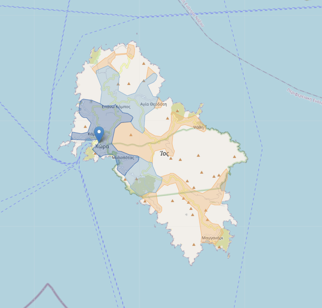
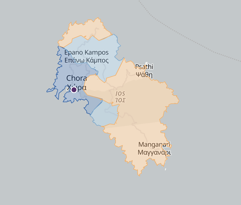
Thus, we transferred the isodistance zone data to QGIS, where we identified areas not covered by the country’s basic road network, and reclassified them as “roadless”. The classification of “basic road network” was done through OSM data, by unifying the entire road network of mainland Greece and it’s islands into one and deleting dozens of small road networks in mountain areas, to identify locations where in reality no normal vehicle would be able to access. We then split these zones according to the nearest neighboring zones that did have a connection to the road network, and assigned them that zone’s category.
Isodistances without code
The approach followed in this article (openrouteservice, QGIS, etc.) is one of the many ways one can approach distance-zone calculation. There are several other tools online, including openrouteservice itself, with which you can visualize distance from a point directly and without getting involved with code or geospatial data processing software. Websites such as iso4app, distance.to or calcmaps can quickly map the proximity of a hospital, a school, or any point on the map.
The geospatial files, the dataset containing all school units across Greece, and a code example used for this data-driven article are openly available in a relevant GitHub repository