Climate data often come up in the newscycle during major weather events. Copernicus data can be analyzed using a few lines of Python code, without installing software or downloading files to your computer.
Translation: This piece was originally written in Greek. It was translated into English with AI assistance and has been reviewed and edited by the author, Pavlos Methodios.
The summer of 2026 in Europe broke previous weather records, with multiple heatwaves and persistent drought. Cities in Western Europe recorded temperatures above 40°C, while France experienced four spells of extreme heat lasting a total of 45 days, according to the Paris Climate Agency. London’s lush green parks looked more like scenes from a Mediterranean country as drought scorched the vegetation. Wildfires reached “record levels” in England and Wales, while fires in France and Spain burned tens of thousands of hectares.
Rising global temperatures are reflected in the Copernicus ERA5 data. The service provides historical records from 1940 onwards and is an important source of climate data. ERA5 is the fifth generation of reanalysis produced by ECMWF (European Centre for Medium-Range Weather Forecasts). Using the laws of physics, it combines model data with actual observations from weather stations into a single global dataset.
As explained on the Copernicus ERA5 website, this principle, known as “data assimilation”, is based on the method used by weather forecasting centres: at regular intervals—every 12 hours at ECMWF—a previous forecast is combined with newly available observations to produce an updated, improved estimate of the state of the atmosphere. This estimate is called an analysis, and an updated, improved forecast is then generated from it. Reanalysis works in the same way but at a reduced resolution, making it possible to provide a historical dataset.
Accessing the data through code
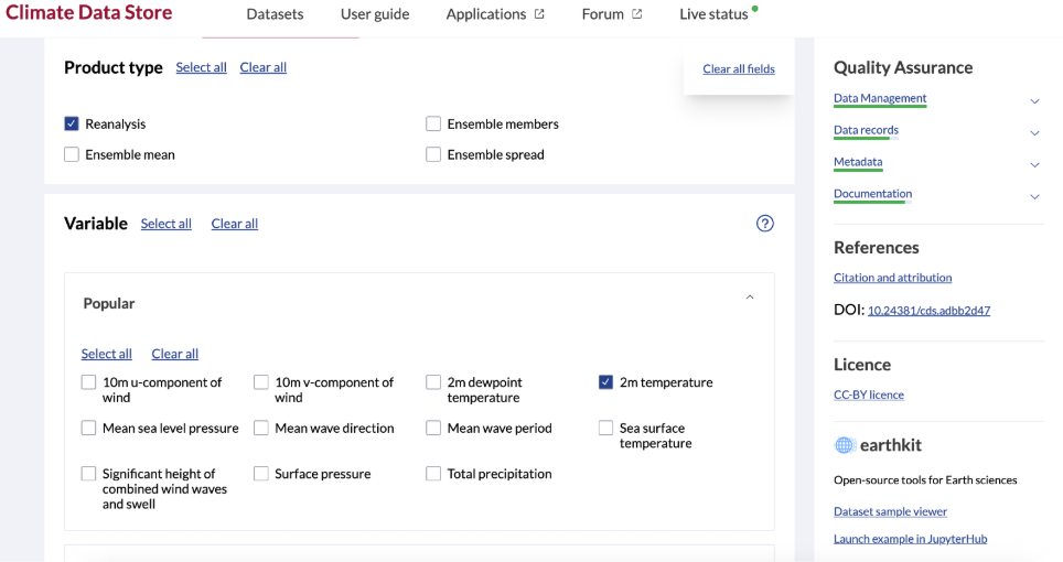
The Copernicus Climate Data Store provides open data on a wide range of topics, from those of broader interest, such as temperature and precipitation, to more specialised subjects, such as ice sheet velocity in Antarctica and Greenland, and upper tropospheric humidity. The data can be accessed through the more conventional method of retrieving them using the service’s online form, selecting options to specify the information to be included in the final file.
For this article, however, we took a different approach: we used ARCO (Analysis Ready Cloud Optimized) data, a repackaged version of the original ERA5 data that provides direct programmatic access, via an API, to a more limited selection of datasets. This removes the need to download them to our device, making it easier to access a broad range of data.
To access the data, you need to create a free Copernicus account to obtain an API key.
In our case, we chose to analyze the data in Google Colab, an open, cloud-based platform for running Python code in a browser, without installing additional software.
In the Python script we wrote, we used ERA5, which provides climate data at a spatial grid resolution of approximately 31 kilometres. We selected this dataset rather than the equivalent ERA5-Land dataset, which offered a finer grid resolution of 9 kilometres, because we frequently needed to visualise areas with complex coastlines, such as islands and peninsulas.
The available parameters range from wind and pressure to temperature and total precipitation, and also include sea surface temperature. In this article, we focused on retrieving temperature and precipitation data, as these two categories have a more direct impact on our daily lives.
| Name | Unit | Variable name | Note |
| 10 metre U wind component | m s-1 | u10 | |
| 100 metre U wind component | m s-1 | u100 | |
| 10 metre V wind component | m s-1 | v10 | |
| 100 metre V wind component | m s-1 | v100 | |
| 10m wind gust since previous post-processing | m s-1 | fg10 | |
| 2 metre dewpoint temperature | K | d2m | |
| 2 metre temperature | K | t2m | |
| Mean sea level pressure | Pa | msl | |
| Sea surface temperature | K | sst | Sea surface temperature is available at the usual times, eg hourly, but its content is only updated once daily. |
| Skin temperature | K | skt | |
| Surface pressure | Pa | sp | |
| Surface latent heat flux | J m-2 | slhf | |
| Surface sensible heat flux | J m-2 | sshf | |
| Surface solar radiation downwards | J m-2 | ssrd | |
| Surface thermal radiation downwards | J m-2 | strd | |
| Total precipitation | m | tp | |
| Total cloud cover | (0 – 1) | tcc | |
| Total sky direct solar radiation at surface | J m-2 | fdir | |
| Cloud base height | m | cbh | |
| Boundary layer height | m | blh |
We also selected the spatially chunked (geochunked) version of the dataset, as our approach involves retrieving data by location, whether for a city or a country. We then used the API key to access the data. You can find the key in your profile on the Copernicus website.
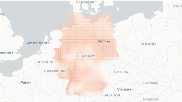
In the code below, we selected Germany as an example and calculated the mean temperature for each year from 1970 to 2025. The country’s boundaries are retrieved using open data from OpenStreetMap and displayed on an interactive map, where users can select the year they want to view.
You do not need to limit yourself to this example. With a few changes to the main variables, you can adjust the parameters and analyze different data.
Script for mapping mean temperature each year in Germany
# –––––––––– SETTINGS - Change the main parameters here ––––––––––––––
variable_name = "t2m"                      # the variable that we want to use
location = "Germany"                        # the country/region that we want to fetch (if not found, check the proper name in OpenStreetMaps)
function = "mean"                          # Options: "mean", "max", "min"
months_list = []                           # Insert months of interest
months = months_list or list(range(1, 13)) # If 'months_list' is empty, it defaults to range(1, 13) covering all 12 months
time_range = range(1970, 2026)             # years of interest

cdsapi_key = "" # Insert your key

# –––––––––––––––––––––––––––––––––––––––––––––––––––––––––––––––––––––

# 0. import libraries
!pip install -q osmnx regionmask flox zarr aiohttp
import os, json
import numpy as np, xarray as xr, geopandas as gpd
import osmnx as ox, regionmask, shapely
import plotly.express as px
from google.colab import userdata


geochunked_url = "https://arco.datastores.ecmwf.int/cadl-arco-geo-002/arco/reanalysis_era5_single_levels/sfc/geoChunked.zarr"
ds = xr.open_zarr(
    geochunked_url,
    consolidated=True,
    storage_options={"headers": {"Authorization": f"Bearer {cdsapi_key}"}},
)


# 1. Boundary
gdf = ox.geocode_to_gdf(location).to_crs("EPSG:4326")
x0, y0, x1, y1 = gdf.total_bounds

# 2. Aggregate per year
cache = f"{location}_{variable_name}_{function}.nc"
if os.path.exists(cache):
    ann = xr.open_dataarray(cache)
else:
    da = ds[variable_name].sel(
        latitude=slice(y1, y0) if ds.latitude[0] > ds.latitude[-1] else slice(y0, y1),
        longitude=slice(x0, x1),
        time=slice(str(time_range[0]), str(time_range[-1])),
    )
    if months_list:  # skip the filter when all months are used
        da = da.sel(time=da.time.dt.month.isin(months))
    ann = getattr(da.groupby("time.year"), function)().compute() - 273.15
    ann.to_netcdf(cache)

# 3. Mask to boundary
mask = regionmask.mask_geopandas(gdf, ann.longitude, ann.latitude)
df = ann.where(mask.notnull()).to_dataframe("temp_c").reset_index().dropna(subset=["temp_c"])
df["temp_c"] = df["temp_c"].round(1)

# 4. Grid cells, clipped to boundary
dy = np.diff(np.unique(df.latitude)).min() / 2
dx = np.diff(np.unique(df.longitude)).min() / 2
cells = df[["latitude", "longitude"]].drop_duplicates().reset_index(drop=True)
cells["cell_id"] = cells.index.astype(str)
grid = gpd.GeoDataFrame(
    cells,
    geometry=shapely.box(cells.longitude - dx, cells.latitude - dy,
                         cells.longitude + dx, cells.latitude + dy),
    crs="EPSG:4326",
)
grid = gpd.clip(grid, gdf)

data = (df.merge(cells, on=["latitude", "longitude"])[["cell_id", "year", "temp_c"]]
          .query("cell_id in @grid.cell_id")
          .sort_values("year"))
data["year"] = data["year"].astype(str)

# 5. Compact geojson + view that fits all polygons
g = grid[["cell_id", "geometry"]].copy()
g["geometry"] = shapely.set_precision(g.geometry.values, 1e-4)
geo = json.loads(g.set_index("cell_id").to_json())

bx0, by0, bx1, by1 = grid.total_bounds
lat_c = (by0 + by1) / 2
zoom = min(np.log2(1000 / 512 * 360 / (bx1 - bx0)),
           np.log2(650 / 512 * 180 / ((by1 - by0) / np.cos(np.radians(lat_c))))) - 0.2

# 6. Figure
unit = function.capitalize()
fig = px.choropleth_map(
    data, geojson=geo, locations="cell_id", color="temp_c", animation_frame="year",
    color_continuous_scale="RdBu_r",
    range_color=[df.temp_c.min() - 5, df.temp_c.max() + 5],
    map_style="carto-positron", zoom=zoom,
    center={"lat": lat_c, "lon": (bx0 + bx1) / 2},
    opacity=0.5,
    labels={"temp_c": f"{unit} Temp (°C)"},
    title=f"{location}: {unit} Temperature by Year (ERA5)",
)
fig.update_traces(marker_line_width=0)
fig.update_layout(margin={"r": 0, "t": 40, "l": 0, "b": 0}, height=650)

for fr in fig.frames:
    for t in fr.data:
        t.geojson = None

OUT = f"/content/{location.lower()}_era5.html"
fig.write_html(OUT, include_plotlyjs="cdn", full_html=True, auto_play=False)
fig.show()
As the visualization for 1970–2025 shows, higher temperatures become increasingly common as we approach 2025, with many areas recording mean annual temperatures above 10°C, according to ERA5.
Annual mean temperature in Germany (1970-2027)
Beyond the country, state or regional level, the data can also provide insights into climate patterns at a smaller geographical scale, such as a particular urban area. In the following code example, we therefore used a list of randomly selected cities and their respective countries or states, and visualised the mean temperatures recorded there during the summer months—June, July and August.
Mean summer temperature for a list of cities
# —————————————————————————————————————————————————————
# SETTINGS — everything a user should change

variable_name = "t2m"                        # ERA5 variable, e.g. "t2m", "tp"
function = "mean"                            # "mean", "max", "min", "sum", "median", "std"
months_list = [6, 7, 8]                            # e.g. [6, 7, 8] for summer only
months = months_list or list(range(1, 13))  # if empty, then gets full year
time_range = range(1970, 2026)              # years of interest

cities = {                                  # city and country/state to find
    "Athens": "Greece",
    "Belgrade": "Serbia",
    "Bologna": "Italy",
    "Burgas": "Bulgaria",
    "Topeka": "Kansas"
}

valid_functions = ["mean", "max", "min", "sum", "median", "std"]

function_labels = {
    "mean": "Mean", "max": "Maximum", "min": "Minimum",
    "sum": "Total", "median": "Median", "std": "Std. dev. of",
}

cdsapi_key = "" # insert your key

# —————————————————————————————————————————————————————

# SETUP: install, import, open the ARCO store
!pip install -q zarr fsspec aiohttp requests plotly xarray

import importlib
import requests
import numpy as np
import pandas as pd
import xarray as xr
import plotly.graph_objects as go
from google.colab import userdata


importlib.invalidate_caches()
xr.backends.plugins.list_engines.cache_clear()
assert "zarr" in xr.backends.list_engines(), "zarr backend still missing, restart the runtime once"


geochunked_url = "https://arco.datastores.ecmwf.int/cadl-arco-geo-002/arco/reanalysis_era5_single_levels/sfc/geoChunked.zarr"

ds = xr.open_zarr(
    geochunked_url,
    consolidated=True,
    storage_options={"headers": {"Authorization": f"Bearer {cdsapi_key}"}},
)

# Unit conversion per variable: (function applied to raw value, display unit)
unit_conversions = {
    "t2m":                      (lambda x: x - 273.15, "°C"),
    "2m_dewpoint_temperature":  (lambda x: x - 273.15, "°C"),
    "skin_temperature":         (lambda x: x - 273.15, "°C"),
    "sea_surface_temperature":  (lambda x: x - 273.15, "°C"),
    "tp":                       (lambda x: x * 1000,   "mm"),  # metres -> mm
}
convert_fn, unit_label = unit_conversions.get(variable_name, (lambda x: x, ""))

# Validation
if function not in valid_functions:
    raise ValueError(f"function must be one of: {valid_functions}")
if not months:
    raise ValueError("At least one month must be selected.")
if any(m < 1 or m > 12 for m in months):
    raise ValueError("months_list must contain values between 1 and 12.")

# OPENSTREETMAP
def geocode_city(city, country):
    """Find city coordinates using OpenStreetMap/Nominatim."""
    response = requests.get(
        "https://nominatim.openstreetmap.org/search",
        params={"q": f"{city}, {country}", "format": "jsonv2", "limit": 1},
        headers={"User-Agent": "ERA5-city-analysis/1.0"},
        timeout=10,
    )
    response.raise_for_status()
    results = response.json()
    if not results:
        raise ValueError(f"Could not find {city}, {country} using OpenStreetMap.")
    return float(results[0]["lat"]), float(results[0]["lon"])


def normalize_longitude(lon):
    """Convert longitude to the convention used by ds (-180..180 or 0..360)."""
    ds_min_lon = float(ds["longitude"].min())
    ds_max_lon = float(ds["longitude"].max())
    if ds_min_lon >= 0 and ds_max_lon > 180:
        return lon % 360
    return ((lon + 180) % 360) - 180


# Find complete calendar years
times = pd.to_datetime(ds["time"].values)
time_df = pd.DataFrame({"time": times})
time_df["year"] = time_df["time"].dt.year

year_start = time_df.groupby("year")["time"].min()
year_end = time_df.groupby("year")["time"].max()

complete_years = [
    year for year in sorted(time_df["year"].unique())
    if year_start.loc[year].normalize() <= pd.Timestamp(year=year, month=1, day=1)
    and year_end.loc[year].normalize() >= pd.Timestamp(year=year, month=12, day=31)
]

selected_years = [y for y in complete_years if y in time_range]
if not selected_years:
    raise ValueError("No complete calendar years found within the selected time_range.")

# Per city
city_results = {}

for city_name, country in cities.items():

    target_lat, target_lon = geocode_city(city_name, country)
    dataset_lon = normalize_longitude(target_lon)

    series = ds[variable_name].sel(latitude=target_lat, longitude=dataset_lon, method="nearest")

    df = series.to_dataframe(name=variable_name).reset_index()
    df["year"] = df["time"].dt.year
    df["month"] = df["time"].dt.month
    df = df[df["year"].isin(selected_years) & df["month"].isin(months)]

    annual = df.groupby("year")[variable_name].agg(function).reset_index()
    annual["value"] = convert_fn(annual[variable_name])

    city_results[city_name] = {"country": country, "annual": annual[["year", "value"]]}

# INTERACTIVE CHART — annual values per city
function_label = function_labels[function]
period_label = "All months" if months == list(range(1, 13)) else "Months: " + ", ".join(str(m) for m in months)

fig = go.Figure()
for city_name, r in city_results.items():
    annual_df = r["annual"]
    fig.add_trace(go.Scatter(
        x=annual_df["year"], y=annual_df["value"], mode="lines", name=city_name,
        hovertemplate=f"Year: %{{x}}<br>{city_name}: %{{y:.2f}}{unit_label}<extra></extra>",
    ))

fig.update_layout(
    title=f"{function_label} annual {variable_name} ({unit_label}) — ERA5<br><sup>{period_label}</sup>",
    xaxis_title="Year",
    yaxis_title=f"{variable_name} ({unit_label})",
    template="plotly_white",
    height=500,
)
fig.show()
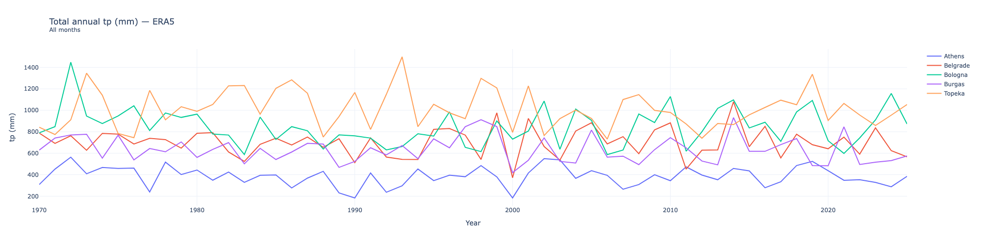
With a few changes to the variables, we can also retrieve total precipitation for each year and each location. In the code above, we change three variables:
- Change
variable_namefrom"t2m"to"tp". - Change
functionfrom"mean"to"sum"to obtain total annual precipitation. - Leave the list of months empty to include every month of the year.
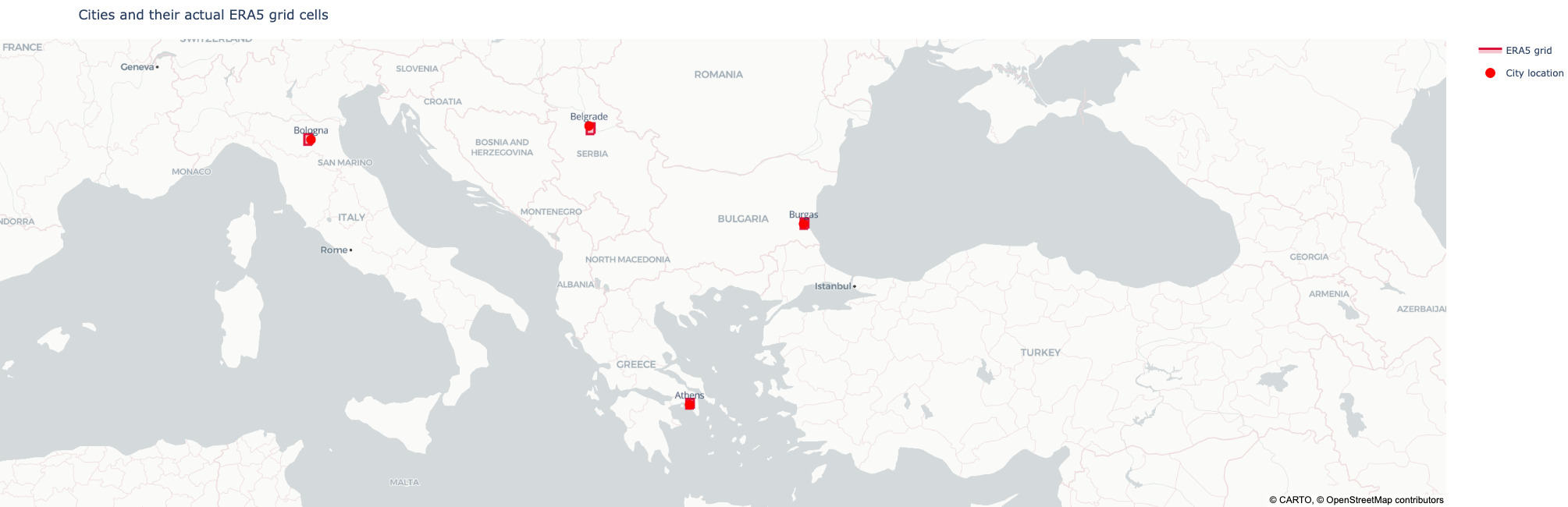
Note that the code automatically selects coordinates based on the city name and its country or state. To verify that we had retrieved data for the intended locations, we plotted the coordinates of the areas for which we had previously obtained historical data on a map.
The full code written and used for this article is available here. In case you prefer to explore the data and not conduct an analysis, you may find useful the ERA Explorer, an online tool by Copernicus that visualizes the historical data for each region of the planet.