
How we grouped 1,602 tennis players to find out who is more similar to Stefanos Tsitsipas and to predict the latter’s career path over the next decade, by applying simple machine learning techniques and statistical methods.
Data collection
What statistics can tell us about Stefanos Tsitsipas’ career
Which players the 22-year-old international is similar with and what are the predictions for his career path over the next decade
Primary data was collected in March 2020 from the Ultimate Tennis Statistics website, which is licensed under a Creative Commons license (CC BY-NC-SA 4.0) and is based on open source software available on GitHub.
More specifically, we collected annual data for the period 2000 to March 2020 from the Association of Tennis Professionals (ATP) world rankings, as published on the Ultimate Tennis Statistics website. We then proceeded to collect profile data published on the same website, regarding 3,912 tennis players included in these rankings.
Indicatively, as can be inferred from Stefanos Tsitsipas’ stats profile on the website, each athlete’s “profile data” includes, among other things, information about the age of the player, the year he turned professional, the seasons he has played, his “backhand“, his favorite surface, the amount of prize money he has earned, the titles he has won, the best rank he has achieved, as well as his current rank, his ELO rank etc.
The aim was to make estimates for the progress of specific players (Stefanos Tsitsipas), using data on the progress of “similar” players. We used the available data to create a single dataset with a set of variables for each player, which we could statistically analyze in order to group athletes based on the degree of similarity with Tsitsipas, and make predictions about their potential career path.
Data cleaning
The constructed dataset can be described as a matrix with p columns and n rows. Each row corresponds to a player and the columns contain the values of the variables that we aim to utilize in order to obtain the desired predictions.
Before conducting any statistical analysis, we computed the proportion of missing values across the dataset’s rows and the columns. We found that in several cases, missing values corresponded to more than 50% of row and column contents. We therefore deleted said rows and columns, since the information they would provide would be negligible. The resulting dataset consisted of 1.602 rows (players) and 20 variables (player names and characteristics). In this dataset, the remaining missing values (those retained after the deletion of rows and columns with missing values in more than 50% of their contents) were imputed by using machine learning techniques and the statistical programming language R.
Dataset sample to be analyzed
| names | prize_money | best_rank | overall_surface_pct | hard_surface_pct | clay_surface_pct | grass_surface_pct | ranksDiff1 | ranksDiff2 | ranksDiff3 | best_rank_std | age_turned_pro | age | plays | backhand | favorite_surface | hard_titles_std | clay_titles_std | titles_std | prize_money_std |
|---|---|---|---|---|---|---|---|---|---|---|---|---|---|---|---|---|---|---|---|
| Feliciano Lopez | 777932.27 | 12 | 0.52 | 0.51 | 0.49 | 0.65 | 112.0 | 97.0 | 34.0 | 18.0 | 15.0 | 38.0 | 2 | 2 | 9 | 0.0909090909090909 | 0.0454545454545455 | 0.31818181818181795 | 13.5643947428156 |
| Nicolas Mahut | 513113.95 | 37 | 0.44 | 0.41 | 0.3 | 0.62 | 172.0 | 53.0 | 175.0 | 14.0 | 18.0 | 38.0 | 3 | 2 | 9 | 0.2 | 13.1482532242432 | ||
| Tommy Robredo | 636963.57 | 5 | 0.6 | 0.56 | 0.66 | 0.54 | 101.0 | 1.0 | 9.0 | 8.0 | 15.0 | 37.0 | 3 | 2 | 4 | 0.0476190476190476 | 0.523809523809524 | 0.5714285714285711 | 13.364467742966001 |
| Paolo Lorenzi | 351977.79 | 33 | 0.38 | 0.36 | 0.42 | 0.2 | 99.0 | 415.0 | 134.0 | 14.0 | 21.0 | 38.0 | 3 | 3 | 15 | 0.0714285714285714 | 0.0714285714285714 | 12.7713233559987 | |
| Ivo Karlovic | 468826.9 | 14 | 0.52 | 0.52 | 0.42 | 0.63 | 93.0 | 8.0 | 128.0 | 8.0 | 21.0 | 41.0 | 3 | 2 | 9 | 0.19047619047619 | 0.0476190476190476 | 0.38095238095238104 | 13.057988896144801 |
| Roger Federer | 5618777.87 | 1 | 0.82 | 0.83 | 0.76 | 0.87 | 16.0 | 7.0 | 4.0 | 6.0 | 16.0 | 38.0 | 3 | 2 | 9 | 3.08695652173913 | 0.4782608695652171 | 4.4782608695652195 | 15.5416247373677 |
| Guillermo Garcia Lopez | 470796.06 | 23 | 0.46 | 0.42 | 0.5 | 0.48 | 501.0 | 132.0 | 115.0 | 9.0 | 18.0 | 36.0 | 3 | 2 | 16 | 0.11764705882352902 | 0.17647058823529396 | 0.294117647058824 | 13.062180285599199 |
| Jo Wilfried Tsonga | 1379538.44 | 5 | 0.68 | 0.68 | 0.64 | 0.69 | 399.0 | 106.0 | 231.0 | 8.0 | 18.0 | 34.0 | 3 | 3 | 6 | 1.0625 | 0.0625 | 1.125 | 14.137259537419801 |
| Fernando Verdasco | 913358.47 | 7 | 0.57 | 0.54 | 0.61 | 0.55 | 291.0 | 64.0 | 73.0 | 8.0 | 17.0 | 36.0 | 2 | 3 | 4 | 0.10526315789473699 | 0.263157894736842 | 0.368421052631579 | 13.724883711215199 |
| Andreas Seppi | 587859.78 | 18 | 0.48 | 0.46 | 0.5 | 0.57 | 444.0 | 113.0 | 94.0 | 11.0 | 18.0 | 36.0 | 3 | 3 | 9 | 0.0555555555555556 | 0.0555555555555556 | 0.166666666666667 | 13.2842437290547 |
| Philipp Kohlschreiber | 674084.05 | 16 | 0.56 | 0.54 | 0.57 | 0.6 | 512.0 | 39.0 | 120.0 | 11.0 | 17.0 | 36.0 | 3 | 2 | 14 | 0.0526315789473684 | 0.315789473684211 | 0.421052631578947 | 13.421110085383699 |
| Teymuraz Gabashvili | 291151.07 | 43 | 0.37 | 0.36 | 0.39 | 0.27 | 71.0 | 596.0 | 23.0 | 15.0 | 15.0 | 34.0 | 3 | 3 | 12 | 12.5815975523401 | |||
| Rafael Nadal | 6294819.0 | 1 | 0.83 | 0.78 | 0.92 | 0.78 | 611.0 | 151.0 | 2.0 | 7.0 | 14.0 | 33.0 | 2 | 3 | 4 | 1.1578947368421102 | 3.1052631578947403 | 4.47368421052632 | 15.655237472068698 |
| Jurgen Melzer | 519159.4 | 8 | 0.51 | 0.51 | 0.52 | 0.53 | 190.0 | 77.0 | 12.0 | 12.0 | 17.0 | 38.0 | 3 | 3 | 2 | 0.2 | 0.05 | 0.25 | 13.159966244087999 |
| Dustin Brown | 264191.91 | 64 | 0.39 | 0.34 | 0.4 | 0.45 | 198.0 | 293.0 | 198.0 | 14.0 | 17.0 | 35.0 | 3 | 3 | 9 | 12.484431049859701 | |||
| Stan Wawrinka | 1877237.72 | 3 | 0.64 | 0.64 | 0.67 | 0.5 | 489.0 | 3.0 | 114.0 | 12.0 | 16.0 | 34.0 | 3 | 2 | 15 | 0.5 | 0.38888888888888895 | 0.8888888888888891 | 14.4453119564572 |
| Richard Gasquet | 953971.42 | 7 | 0.63 | 0.62 | 0.62 | 0.67 | 68.0 | 14.0 | 91.0 | 5.0 | 15.0 | 33.0 | 3 | 2 | 9 | 0.421052631578947 | 0.157894736842105 | 0.7894736842105259 | 13.7683889919104 |
| David Ferrer | 1749106.17 | 3 | 0.66 | 0.64 | 0.7 | 0.63 | 197.0 | 150.0 | 12.0 | 13.0 | 17.0 | 37.0 | 3 | 3 | 4 | 0.666666666666667 | 0.7222222222222221 | 1.5 | 14.3746154554174 |
| Go Soeda | 135495.27 | 47 | 0.38 | 0.37 | 0.31 | 0.24 | 249.0 | 133.0 | 200.0 | 35.0 | 3 | 3 | 3 | 11.816692010943502 | |||||
| Carlos Berlocq | 296433.93 | 37 | 0.41 | 0.33 | 0.46 | 0.25 | 292.0 | 364.0 | 10.0 | 11.0 | 18.0 | 37.0 | 3 | 2 | 4 | 0.14285714285714302 | 0.14285714285714302 | 12.5995796395367 | |
| Marcel Granollers | 772940.57 | 19 | 0.45 | 0.41 | 0.48 | 0.45 | 445.0 | 119.0 | 110.0 | 9.0 | 16.0 | 33.0 | 3 | 3 | 16 | 0.0714285714285714 | 0.214285714285714 | 0.28571428571428603 | 13.5579574423371 |
| Gilles Muller | 315361.79 | 21 | 0.52 | 0.53 | 0.46 | 0.56 | 305.0 | 280.0 | 60.0 | 16.0 | 17.0 | 36.0 | 2 | 3 | 6 | 0.0526315789473684 | 0.10526315789473699 | 12.661475798423199 | |
| Dudi Sela | 259822.33 | 29 | 0.42 | 0.45 | 0.19 | 0.48 | 214.0 | 49.0 | 138.0 | 7.0 | 16.0 | 34.0 | 3 | 2 | 6 | 12.4677533302564 | |||
| Daniel Gimeno Traver | 227631.36 | 48 | 0.36 | 0.25 | 0.42 | 0.1 | 619.0 | 12.0 | 75.0 | 9.0 | 18.0 | 34.0 | 3 | 3 | 4 | 12.3354827573315 | |||
| Julien Benneteau | 530930.11 | 25 | 0.48 | 0.49 | 0.41 | 0.47 | 149.0 | 18.0 | 115.0 | 14.0 | 18.0 | 38.0 | 3 | 3 | 3 | 13.182385671975801 | |||
| Novak Djokovic | 1 | 0.83 | 0.84 | 0.8 | 0.84 | 493.0 | 108.0 | 62.0 | 8.0 | 15.0 | 32.0 | 3 | 3 | 6 | 3.4705882352941204 | 0.823529411764706 | 4.64705882352941 | ||
| Yen Hsun Lu | 282170.35 | 33 | 0.42 | 0.42 | 0.24 | 0.44 | 351.0 | 2.0 | 103.0 | 9.0 | 17.0 | 36.0 | 3 | 3 | 6 | 12.5502662455528 | |||
| Viktor Troicki | 575913.2 | 12 | 0.52 | 0.53 | 0.51 | 0.52 | 181.0 | 449.0 | 126.0 | 5.0 | 20.0 | 34.0 | 3 | 3 | 2 | 0.2 | 0.2 | 13.263712233878 | |
| Florian Mayer | 485266.13 | 18 | 0.48 | 0.44 | 0.5 | 0.59 | 480.0 | 143.0 | 215.0 | 10.0 | 17.0 | 36.0 | 3 | 3 | 9 | 0.0666666666666667 | 0.133333333333333 | 13.0924527410764 | |
| Rogerio Dutra Silva | 166942.0 | 63 | 0.32 | 0.29 | 0.36 | 0.01 | 138.0 | 144.0 | 351.0 | 14.0 | 19.0 | 36.0 | 3 | 2 | 15 | 12.025401725685198 | |||
| Janko Tipsarevic | 506824.94 | 8 | 0.53 | 0.54 | 0.52 | 0.53 | 453.0 | 22.0 | 44.0 | 10.0 | 17.0 | 35.0 | 3 | 3 | 2 | 0.17647058823529396 | 0.0588235294117647 | 0.23529411764705901 | 13.1359209369523 |
| Ruben Ramirez Hidalgo | 167582.5 | 50 | 0.34 | 0.19 | 0.39 | 0.01 | 179.0 | 13.0 | 61.0 | 8.0 | 20.0 | 42.0 | 3 | 3 | 4 | 12.029231046304 | |||
| Mischa Zverev | 403370.93 | 25 | 0.4 | 0.41 | 0.32 | 0.5 | 35.0 | 26.0 | 444.0 | 12.0 | 17.0 | 32.0 | 2 | 3 | 9 | 0.0714285714285714 | 12.9076118394366 | ||
| Mikhail Youzhny | 713222.5 | 8 | 0.54 | 0.55 | 0.51 | 0.57 | 55.0 | 26.0 | 11.0 | 9.0 | 16.0 | 37.0 | 3 | 2 | 3 | 0.3 | 0.15 | 0.5 | 13.477548712426401 |
| Gael Monfils | 1054753.88 | 6 | 0.64 | 0.66 | 0.61 | 0.59 | 686.0 | 209.0 | 16.0 | 12.0 | 17.0 | 33.0 | 3 | 3 | 10 | 0.529411764705882 | 0.0588235294117647 | 0.588235294117647 | 13.8688180085766 |
| Andy Murray | 4102933.8 | 1 | 0.77 | 0.78 | 0.7 | 0.84 | 129.0 | 347.0 | 47.0 | 11.0 | 17.0 | 32.0 | 3 | 3 | 9 | 2.2666666666666697 | 0.2 | 3.06666666666667 | 15.227212836758499 |
| Marco Chiudinelli | 134908.0 | 52 | 0.35 | 0.35 | 0.26 | 0.4 | 16.0 | 109.0 | 33.0 | 10.0 | 18.0 | 38.0 | 3 | 3 | 3 | 11.812348343624999 | |||
| Marcos Baghdatis | 557432.31 | 8 | 0.56 | 0.57 | 0.43 | 0.58 | 376.0 | 38.0 | 104.0 | 3.0 | 17.0 | 34.0 | 3 | 3 | 6 | 0.1875 | 0.25 | 13.2310963579044 | |
| Gilles Simon | 869037.88 | 6 | 0.58 | 0.58 | 0.58 | 0.57 | 310.0 | 53.0 | 79.0 | 7.0 | 17.0 | 35.0 | 3 | 3 | 2 | 0.529411764705882 | 0.294117647058824 | 0.823529411764706 | 13.675141993631199 |
| Sergiy Stakhovsky | 314649.47 | 31 | 0.45 | 0.46 | 0.38 | 0.48 | 198.0 | 151.0 | 11.0 | 7.0 | 17.0 | 34.0 | 3 | 2 | 6 | 0.17647058823529396 | 0.23529411764705901 | 12.659214504542401 | |
| Simone Bolelli | 360726.07 | 36 | 0.43 | 0.36 | 0.48 | 0.52 | 354.0 | 19.0 | 123.0 | 6.0 | 17.0 | 34.0 | 3 | 2 | 16 | 12.7958741404096 | |||
| Stephane Robert | 218865.73 | 50 | 0.34 | 0.36 | 0.31 | 0.33 | 573.0 | 103.0 | 27.0 | 15.0 | 20.0 | 39.0 | 3 | 3 | 2 | 12.2962137157501 | |||
| Radek Stepanek | 597024.42 | 8 | 0.56 | 0.56 | 0.55 | 0.6 | 265.0 | 479.0 | 17.0 | 10.0 | 17.0 | 41.0 | 3 | 3 | 2 | 0.263157894736842 | 0.263157894736842 | 13.299713296060801 | |
| Jaroslav Pospisil | 179194.67 | 103 | 0.12 | 0.33 | 0.01 | 0.01 | 157.0 | 99.0 | 338.0 | 39.0 | 3 | 1 | 1 | 12.096228035777099 | |||||
| Lukasz Kubot | 590473.08 | 41 | 0.43 | 0.36 | 0.47 | 0.5 | 147.0 | 13.0 | 69.0 | 8.0 | 19.0 | 37.0 | 3 | 3 | 16 | 13.288679325096 | |||
| Jan Mertl | 300402.5 | 163 | 0.67 | 0.99 | 0.5 | 87.0 | 52.0 | 229.0 | 5.0 | 20.0 | 38.0 | 3 | 1 | 1 | 12.6128785210745 | ||||
| Daniel Munoz De La Nava | 138074.38 | 68 | 0.24 | 0.3 | 0.22 | 205.0 | 241.0 | 276.0 | 17.0 | 17.0 | 38.0 | 2 | 3 | 10 | 11.835547804446099 | ||||
| Frank Dancevic | 117914.62 | 65 | 0.38 | 0.38 | 0.05 | 0.48 | 233.0 | 30.0 | 17.0 | 4.0 | 18.0 | 35.0 | 3 | 2 | 3 | 11.6777160822304 | |||
| Lamine Ouahab | 38605.17 | 114 | 0.5 | 0.38 | 0.53 | 361.0 | 76.0 | 114.0 | 7.0 | 17.0 | 35.0 | 3 | 3 | 4 | 10.561141484307901 | ||||
| Giovanni Lapentti | 49029.0 | 110 | 0.34 | 0.46 | 0.24 | 0.33 | 505.0 | 142.0 | 149.0 | 3.0 | 19.0 | 37.0 | 3 | 3 | 10 | 10.8001672387612 | |||
| Fabio Fognini | 841913.38 | 9 | 0.54 | 0.48 | 0.59 | 0.51 | 415.0 | 58.0 | 152.0 | 15.0 | 16.0 | 32.0 | 3 | 3 | 4 | 0.0625 | 0.5 | 0.5625 | 13.643432413823302 |
| Flavio Cipolla | 203031.25 | 70 | 0.35 | 0.38 | 0.36 | 0.12 | 319.0 | 51.0 | 70.0 | 9.0 | 19.0 | 36.0 | 3 | 2 | 15 | 12.2211151870629 | |||
| Filippo Volandri | 263308.73 | 25 | 0.44 | 0.13 | 0.54 | 0.15 | 48.0 | 60.0 | 106.0 | 10.0 | 15.0 | 38.0 | 3 | 2 | 4 | 0.133333333333333 | 0.133333333333333 | 12.4810825010305 | |
| Santiago Giraldo | 61.57 | 28 | 0.45 | 0.39 | 0.51 | 0.43 | 390.0 | 152.0 | 34.0 | 8.0 | 18.0 | 32.0 | 3 | 3 | 4 | 4.12017473892312 | |||
| Adrian Menendez Maceiras | 199829.83 | 111 | 0.25 | 0.29 | 0.17 | 0.25 | 298.0 | 76.0 | 208.0 | 10.0 | 19.0 | 34.0 | 3 | 3 | 10 | 12.2052214333519 | |||
| Jan Hernych | 143583.67 | 59 | 0.4 | 0.42 | 0.32 | 0.48 | 93.0 | 35.0 | 34.0 | 11.0 | 18.0 | 40.0 | 3 | 3 | 9 | 11.8746732104669 | |||
| Maximo Gonzalez | 203559.91 | 58 | 0.32 | 0.19 | 0.37 | 0.01 | 50.0 | 250.0 | 265.0 | 7.0 | 18.0 | 36.0 | 3 | 3 | 4 | 12.2237156385726 | |||
| Michal Przysiezny | 103031.92 | 57 | 0.29 | 0.28 | 0.21 | 0.33 | 50.0 | 135.0 | 107.0 | 13.0 | 17.0 | 36.0 | 3 | 2 | 3 | 11.542794122114401 | |||
| Albert Montanes | 345078.82 | 22 | 0.47 | 0.3 | 0.53 | 0.32 | 109.0 | 13.0 | 3.0 | 11.0 | 18.0 | 39.0 | 3 | 3 | 4 | 0.3529411764705879 | 0.3529411764705879 | 12.7515281336877 | |
| Nicolas Almagro | 672014.62 | 9 | 0.59 | 0.47 | 0.66 | 0.47 | 106.0 | 582.0 | 53.0 | 8.0 | 17.0 | 34.0 | 3 | 2 | 4 | 0.8125 | 0.8125 | 13.418035375220999 | |
| Konstantin Kravchuk | 114634.22 | 78 | 0.26 | 0.22 | 0.5 | 0.2 | 28.0 | 295.0 | 2.0 | 12.0 | 19.0 | 35.0 | 3 | 3 | 14 | 11.649501642529 | |||
| Lleyton Hewitt | 1043996.7 | 1 | 0.7 | 0.7 | 0.64 | 0.76 | 6.0 | 1.0 | 16.0 | 3.0 | 17.0 | 39.0 | 3 | 3 | 9 | 1.0 | 0.1 | 1.5 | 13.8585668865002 |
| Tomas Berdych | 1734784.0 | 4 | 0.65 | 0.65 | 0.63 | 0.68 | 285.0 | 68.0 | 21.0 | 13.0 | 16.0 | 34.0 | 3 | 3 | 14 | 0.529411764705882 | 0.11764705882352902 | 0.7647058823529409 | 14.3663934679356 |
| Igor Sijsling | 216377.5 | 52 | 0.36 | 0.35 | 0.3 | 0.44 | 101.0 | 481.0 | 83.0 | 9.0 | 17.0 | 32.0 | 3 | 2 | 9 | 12.284779846426801 | |||
| Teodor Dacian Craciun | 218 | 141.0 | 253.0 | 51.0 | 9.0 | 17.0 | 39.0 | 3 | 3 | 1 | |||||||||
| Denis Istomin | 372861.12 | 33 | 0.47 | 0.46 | 0.45 | 0.54 | 662.0 | 4.0 | 30.0 | 8.0 | 17.0 | 33.0 | 3 | 3 | 9 | 0.0625 | 0.125 | 12.8289612968533 | |
| Steve Darcis | 220764.13 | 38 | 0.47 | 0.47 | 0.47 | 0.46 | 114.0 | 215.0 | 330.0 | 14.0 | 18.0 | 35.0 | 3 | 2 | 2 | 0.0666666666666667 | 0.0666666666666667 | 0.133333333333333 | 12.3048501254777 |
| Kevin Anderson | 1163846.71 | 5 | 0.59 | 0.61 | 0.53 | 0.59 | 101.0 | 249.0 | 296.0 | 11.0 | 20.0 | 33.0 | 3 | 3 | 6 | 0.42857142857142894 | 0.42857142857142894 | 13.9672412061614 | |
| Dmitry Tursunov | 394675.0 | 20 | 0.51 | 0.52 | 0.4 | 0.57 | 146.0 | 146.0 | 222.0 | 6.0 | 17.0 | 37.0 | 3 | 3 | 3 | 0.33333333333333304 | 0.46666666666666706 | 12.8858179203999 | |
| Michael Berrer | 212823.15 | 42 | 0.38 | 0.41 | 0.3 | 0.29 | 127.0 | 152.0 | 26.0 | 11.0 | 18.0 | 39.0 | 2 | 2 | 10 | 12.2682168181267 | |||
| Tobias Kamke | 216612.27 | 64 | 0.38 | 0.37 | 0.36 | 0.46 | 93.0 | 271.0 | 235.0 | 7.0 | 17.0 | 33.0 | 3 | 3 | 9 | 12.285864260144 | |||
| Paul Henri Mathieu | 370534.88 | 12 | 0.48 | 0.46 | 0.49 | 0.42 | 125.0 | 114.0 | 47.0 | 9.0 | 17.0 | 38.0 | 3 | 3 | 3 | 0.11764705882352902 | 0.23529411764705901 | 12.822702862337 | |
| Frederico Gil | 145393.3 | 62 | 0.47 | 0.39 | 0.55 | 0.12 | 344.0 | 125.0 | 10.0 | 8.0 | 17.0 | 34.0 | 3 | 3 | 4 | 11.8871977632399 | |||
| Malek Jaziri | 294278.0 | 42 | 0.41 | 0.42 | 0.43 | 0.3 | 168.0 | 201.0 | 158.0 | 16.0 | 19.0 | 36.0 | 3 | 3 | 15 | 12.5922801777746 | |||
| Ernests Gulbis | 453547.06 | 10 | 0.51 | 0.5 | 0.52 | 0.38 | 277.0 | 80.0 | 8.0 | 10.0 | 15.0 | 31.0 | 3 | 3 | 3 | 0.3125 | 0.0625 | 0.375 | 13.024854313826099 |
| Sam Querrey | 794143.47 | 11 | 0.56 | 0.56 | 0.45 | 0.64 | 485.0 | 67.0 | 24.0 | 12.0 | 18.0 | 32.0 | 3 | 3 | 9 | 0.5333333333333329 | 0.0666666666666667 | 0.666666666666667 | 13.5850194166015 |
| Blaz Kavcic | 163640.09 | 68 | 0.39 | 0.37 | 0.42 | 0.2 | 458.0 | 60.0 | 106.0 | 7.0 | 18.0 | 33.0 | 3 | 3 | 15 | 12.005424722031 | |||
| Toshihide Matsui | 98480.67 | 261 | 0.67 | 0.6 | 237.0 | 72.0 | 223.0 | 41.0 | 3 | 3 | 1 | 11.4976155642471 | |||||||
| Juan Monaco | 577459.79 | 10 | 0.56 | 0.46 | 0.63 | 0.39 | 315.0 | 146.0 | 251.0 | 10.0 | 17.0 | 35.0 | 3 | 3 | 4 | 0.0714285714285714 | 0.5714285714285711 | 0.6428571428571429 | 13.2663940912483 |
| Robin Haase | 508178.29 | 33 | 0.46 | 0.44 | 0.51 | 0.4 | 502.0 | 53.0 | 2.0 | 7.0 | 17.0 | 32.0 | 3 | 3 | 4 | 0.14285714285714302 | 0.14285714285714302 | 13.1385876295539 | |
| Michael Russell | 156858.0 | 60 | 0.34 | 0.37 | 0.26 | 0.3 | 68.0 | 70.0 | 345.0 | 9.0 | 19.0 | 41.0 | 3 | 3 | 10 | 11.9630962164622 | |||
| Jimmy Wang | 87971.23 | 85 | 0.46 | 0.46 | 0.29 | 0.39 | 516.0 | 197.0 | 26.0 | 5.0 | 16.0 | 35.0 | 3 | 3 | 3 | 11.3847651081883 | |||
| Lukas Lacko | 232969.07 | 44 | 0.4 | 0.42 | 0.2 | 0.42 | 190.0 | 92.0 | 186.0 | 8.0 | 17.0 | 32.0 | 3 | 3 | 6 | 12.358660976955099 | |||
| Tommy Haas | 680499.35 | 2 | 0.63 | 0.64 | 0.59 | 0.63 | 15.0 | 3.0 | 6.0 | 6.0 | 17.0 | 41.0 | 3 | 2 | 2 | 0.55 | 0.1 | 0.75 | 13.430582145893199 |
| Pablo Andujar | 411965.85 | 32 | 0.41 | 0.29 | 0.51 | 0.12 | 611.0 | 146.0 | 69.0 | 11.0 | 18.0 | 34.0 | 3 | 3 | 4 | 0.307692307692308 | 0.307692307692308 | 12.9286957365467 | |
| Adrian Mannarino | 531070.77 | 22 | 0.46 | 0.46 | 0.26 | 0.59 | 457.0 | 122.0 | 190.0 | 14.0 | 15.0 | 31.0 | 2 | 3 | 9 | 0.0769230769230769 | 13.1826505681797 | ||
| Matthias Bachinger | 142133.73 | 85 | 0.36 | 0.39 | 0.37 | 0.22 | 316.0 | 159.0 | 52.0 | 6.0 | 17.0 | 32.0 | 3 | 3 | 15 | 11.8645236539685 | |||
| Lukas Rosol | 300705.64 | 26 | 0.44 | 0.39 | 0.52 | 0.4 | 328.0 | 17.0 | 89.0 | 10.0 | 18.0 | 34.0 | 3 | 3 | 4 | 0.0714285714285714 | 0.0714285714285714 | 0.14285714285714302 | 12.613887125036198 |
| Jeremy Chardy | 577229.53 | 25 | 0.5 | 0.48 | 0.53 | 0.48 | 303.0 | 69.0 | 117.0 | 8.0 | 18.0 | 33.0 | 3 | 3 | 2 | 0.0666666666666667 | 0.0666666666666667 | 13.2659952653493 | |
| Matteo Viola | 123883.8 | 118 | 0.24 | 0.33 | 0.01 | 0.01 | 142.0 | 154.0 | 402.0 | 9.0 | 16.0 | 32.0 | 3 | 3 | 10 | 11.727099308463302 | |||
| Marc Fornell Mestres | 236 | 0.01 | 0.01 | 94.0 | 178.0 | 66.0 | 38.0 | 3 | 1 | 1 | |||||||||
| Pablo Cuevas | 530023.94 | 19 | 0.53 | 0.41 | 0.6 | 0.41 | 480.0 | 124.0 | 117.0 | 12.0 | 18.0 | 34.0 | 3 | 2 | 4 | 0.375 | 0.375 | 13.1806774543195 | |
| Potito Starace | 315379.17 | 27 | 0.46 | 0.31 | 0.53 | 0.08 | 84.0 | 200.0 | 33.0 | 6.0 | 19.0 | 38.0 | 3 | 3 | 4 | 12.6615309082103 | |||
| Victor Hanescu | 306932.21 | 26 | 0.45 | 0.34 | 0.54 | 0.41 | 265.0 | 40.0 | 102.0 | 10.0 | 17.0 | 38.0 | 3 | 2 | 4 | 0.0714285714285714 | 0.0714285714285714 | 12.634382187854 | |
| Ivo Klec | 68838.17 | 184 | 0.22 | 0.2 | 0.25 | 282.0 | 309.0 | 264.0 | 7.0 | 18.0 | 39.0 | 3 | 3 | 1 | 11.1395136665904 | ||||
| Leonardo Mayer | 499417.46 | 21 | 0.48 | 0.43 | 0.53 | 0.46 | 453.0 | 67.0 | 64.0 | 12.0 | 15.0 | 32.0 | 3 | 2 | 4 | 0.153846153846154 | 0.153846153846154 | 13.121197618171001 | |
| Carlos Salamanca | 55554.83 | 137 | 0.38 | 0.01 | 0.75 | 197.0 | 48.0 | 446.0 | 9.0 | 18.0 | 37.0 | 2 | 3 | 1 | 10.9251257399828 | ||||
| Donald Young | 308544.0 | 38 | 0.4 | 0.42 | 0.22 | 0.38 | 59.0 | 394.0 | 38.0 | 8.0 | 14.0 | 30.0 | 2 | 3 | 6 | 12.639619737765301 | |||
| Alejandro Falla | 193833.19 | 50 | 0.4 | 0.39 | 0.43 | 0.39 | 291.0 | 148.0 | 104.0 | 12.0 | 16.0 | 36.0 | 2 | 3 | 2 | 12.1747532228056 |
Handling missing values
Imputation of missing values
#clear the R environment
rm(list = ls())
#load the MissForest R library to impute the dataset
library(missForest)
#read data for imputation
cleaned_data = read.csv("cleaned_raw_data.csv")
#remove some unused variables
mydata = cleaned_data[,2:6,8:10]
#log and logit transformations when needed
mydata[,c(1:2)] = log(mydata[,1:2])
mydata[,c(3:5)] =log(mydata[,c(3:5)]/(1-mydata[,c(3:5)]))
#impute missing values
mydata.imp <- missForest(mydata)$ximp
In order to impute the remaining missing values of the dataset, the missForest R package was used (see MissForest —non-parametric missing value imputation for mixed-type data). It is a machine learning method based on the Random Forest algorithm, which can briefly be described as a bunch of “decision trees” bundled together.
Random Forest can be explained with the following simple example: let us consider we have a sample of people whose gender is unknown to us (missing value) and that we wish to predict it based on their height and weight data, which we already have. We construct a “decision tree” with two “nodes” for this simple working hypothesis: The first node consists of a question regarding the height of each person and, if the height is greater than 1.80 m, the person is classified as “man”. Conversely, if the person’s height is less than 1.80 m, we move on to the second node – which is made up of a question about the weight of the person – in order to decide: if the person weighs less than 70 kg, they are classified as “woman”. In more complicated examples, the number of nodes is increased and a large number of decision trees can be combined in order to make the desired prediction.
In the case of missing values, we essentially end up with estimated values, with which the missing ones are replaced, training the algorithm by feeding it available data. In this dataset, on which the statistical analysis for the specific story is based, we have included a common list of characteristics for each player (ranking positions, prize rewards, “backhand”, favorite surface, age turned professional, etc.). Each characteristic is a variable, i.e. a column in the dataset.
Let us assume we lack data on a player’s prize money. We have:
- missing values for prize money received by player a
- available values for other characteristics of player a
- υφιστάμενες τιμές για κάποια από τα χαρακτηριστικά της λίστας, στην περίπτωση άλλων αθλητών
- missing values for other characteristics on the list, in the case of other players
We classify the characteristics of players (variables), based on the number of missing values occurring in their dataset in ascending order – starting with the player with the most complete dataset and finishing with the one with the most incomplete one.
Based on this classification, missing values for each player x and for each of his characteristics (variables) are imputed by using the Random Forest algorithm, which is based on: a) available values for other characteristics of player x and b) available values of other players for the characteristic that player x has a missing value. A similar process is followed for each variable containing missing values and repeated several times, until it meets specific performance criteria.
Finding similarities between players
Clustering players by similarity and selecting Tsitsipas’ cluster
#clear the R environment
rm(list = ls())
#load R libraries
library(missForest)
library(KRLS)#to compute RBF
library(irlba) #to compute partial eigen decomposition
library(spam)#to facilitate linear algebra computations
library(spam64)#to facilitate linear algebra computations

#read and clean the data
cleaned_data = read.csv("cleaned_raw_data.csv")
names = cleaned_data$names
mydata = cleaned_data[,2:6,8:10]

#log and logit transformations
mydata[,c(1:2)] = log(mydata[,1:2])
mydata[,c(3:5)] =log(mydata[,c(3:5)]/(1-mydata[,c(3:5)]))

#impute missing values
mydata.imp <- missForest(mydata)$ximp

#compute similarity matrix
mysimils =gausskernel(mydata.imp, sigma=1) #introduce sparsity to facilitate linear algebra computations by setting low similarities equal to 0
mysimils[which(mysimils<=10^(-5))]=0

#compute regularized Laplacian of similarity matrix
diag(mysimils) =0
N= dim(mysimils)[1]
DD = rep(NA,N)
for(i in 1:N) DD[i] = sum(mysimils[i,])

DD = DD + mean(DD)
myd =diag.spam(1/sqrt(DD))
tSimils =myd%*%mysimils%*%myd

#compute partial spectral decomposition of Laplacian
K=150
myeigen = partial_eigen(as.dgCMatrix.spam(tSimils), n =K, symmetric = TRUE)
U = myeigen$vectors

#normalize eigenvectors to have unit length
scalar1 <- function(x) {x / sqrt(sum(x^2))}
Ustar = matrix(NA,dim(U)[1],dim(U)[2])
for(i in 1:dim(U)[1]){
  Ustar[i,] = scalar1(U[i,])

#run k-means
km = kmeans(Ustar,centers = 150,iter.max = 1000)

#find Tsitsipas cluster
size_clsts = km$size
clsts = which(size_clsts>=2)
same_players =list()
tsitsipas_clst=rep(0,length(clsts))
for(i in 1:length(clsts)){
  same_players[[i]] =  which( km$cluster==clsts[i] )
  if(length(  intersect(same_players[[i]],which(names=="Stefanos Tsitsipas")))>0)
  {
    tsitsipas_clst[i] = 1
  }
}
select_tsitsip_clst = same_players[[which(tsitsipas_clst>0)]]
select_tsitsip_clst=select_tsitsip_clst[-5] #we exclude the fifth member of the cluster because he seems to be an outlier due to two injuries that he had and he stopped and started again
tsitsipas_clst_data = cleaned_data[select_tsitsip_clst,]
tsitsipas_clst_names = names[select_tsitsip_clst]
After replacing the missing values, the dataset of 1.602 rows (each player, one row) and 20 columns (each column, one player characteristic) was completed. For each possible pair of players, a similarity index was calculated, using the “radial base function” (RBF kernel). This similarity index is a positive number informing us about the degree of similarity between a player and any athlete in the dataset.
Subsequently, a “similarity matrix” is created, i.e. a matrix that integrates this similarity index to compare coupled players. It is a 1,602 x 1,602 table – rows and columns correspond to the study’s players, thus forming the possible pairs of players: in each cell of the similarity matrix, there is a value that corresponds to the similarity index between the two reference tennis players.
Next, in order for players who are similar to each other to be categorized in groups, we adopt the cluster analysis technique and, in particular, the technique of spectral clustering – the similarity matrix is quite large (1,602 x 1,602) and it would be easier to work with a matrix of smaller dimensions, which, however, would contain as much information as possible from the original similarity matrix.
We follow these steps:
- Original similarity matrix transformation to a normalized Laplacian matrix
- Laplacian matrix principal component analysis (spectral decomposition)
- Grouping rows (players) of the original similarity matrix by applying the k-means algorithm to the spectral decomposition result.
We end up with 150 clusters of similar players and we choose the one Stefanos Tsitsipas belongs to, in order to work on predictions for the player’s ranks.
In fact, the cluster Tsitsipas – whose professional career spans five years now – belongs to, includes players who have had at least 15 years of experience. This is crucial for the prediction method, precisely because our prediction technique is based on pre-existing career paths of similar players.
Predictions method
Considering that the research question is “what world ranking positions Stefanos Tsitsipas might occupy in the future” and given that he has been a professional player for the last five years, we created a prediction model over a ten-year horizon by applying the statistical technique of the sample mean.
We predict the player’s performance over the next ten years, based on the average performance of similar players, who, however, have longer career spans.
In other words, we use actual ranking data of players Tsitsipas is most comparable with, based on their performance after a ten and a 15-year old career path, in order to create estimates for Tsitsipas’ performance over the next decade.
In order for the sample mean (that is, our prediction) not to be affected by any outliers and despite the fact that the Tsitsipas cluster consists of only ten members (himself and nine more players), we are looking for sub-groups of similar athletes within the cluster Stefanos Tsitsipas was assigned to. By computing the Euclidean distance of each player from the centroid of the cluster (as calculated by the k-means algorithm itself), we find:
- sub-group of players a, which is located farther from the centroid of the cluster – these are players who tend to rank slightly better compared to the average positions held by the players of this category during each season. Stefanos Tsitsipas also appears in sub-group a.
- sub-group of players b, which is close to the centroid of the cluster – that is, players whose world ranking positions are close to the average positions held by all players of the category in a given season
In this context, players belonging to the Tsitsipas cluster are selected from these two different sub-groups for test applications of the prediction model: by using data on the first five years of their career, we make “pseudo predictions” for their career path over the next years, which we compare to the actual data on their world ranking. In this way, the margin of error of our predictions emerges.
More specifically, for the purposes of testing the model, the following are selected:
- Alexander Zverev, who, despite having only turned professional seven years ago, belongs to sub-group a (like Stefanos Tsitsipas). He also has a very similar trajectory to Tsitsipas and is one of his major rivals today.
- Stan Wawrinka, David Ferrer and Thomas Berdych, who, on the one hand, have more than 15 years of professional experience and, on the other, belong to sub-group b
For Zverev (sub-group a), the test is applied using a sample mean that results only from the positions held by the cluster’s four players, who are the top-ranked players in a given season. For Wawrinka, Ferrer and Berdych (subgroup b), the “pseudo predictions” are made by calculating the sample mean of the total data pertaining to the cluster players in each season.
As shown in the graph below, the actual ranking of players is usually within our model’s prediction intervals.
For the predictions of Stefanos Tsitsipas’ world ranking performance in the next decade, the prediction method that was applied in the very similar case of Zverev is chosen: for the calculation of the sample mean, lower ranked players compared to the cluster median are excluded and the model takes into account the positions held by the top performing players each time.
Taking a closer look at Zverev’s case and the extent to which the chosen method of calculating the predictions affects the estimated trajectory of Tsitsipas, it is worth noting the following:
Although Zverev finished his sixth professional year ranked No 4., the model had predicted he would have come in 11th (mean prediction) in the respective season, which coincides with the first season of prediction. On the contrary, in the following seasons, the prediction model is “aligned” with Zverev’s actual achievements. The “failure” of the first prediction is explained, if one takes into account that Zverev’s trajectory is similar to that of the other players in the group after the third season of his career. The rapid ascent in world rankings, which characterized both Zverev and Tsitsipas in the first years of their career, is not observed in the case of otherwise identical athletes, whose data, however, “feeds” the model and affects the estimated value for the first prediction season.
It should be noted that a multivariate modelling strategy would be useful for making even more realistic predictions, which is why we suggest this strategy is applied in future studies: in tennis, an athlete’s trajectory significantly depends on their opponents’ progress. In the present model, the working hypothesis is that a player (p) will follow a similar trajectory as his peers’ (n), but it is not assumed that his opponents will have a similar performance to his peers’ (n) opponents considered here.
Data visualization
Charts that visualize statistical data analysis were created using the Python programming language and the statistical programming language R.
More specifically, the Plotly Python Open Source Graphing Library was used to create interactive charts, while static graphs were created using the ggplot2 package in R.
We especially chose to visualize the Tsitsipas cluster and the similarities between the cluster’s players using a radar plot: radar plots are two dimensional charts suitable for the comparative visualization of multiple (quantitative) variables. Especially when more than one case study is visualized, it is the shape of the radar plot that serves the purpose of the visual comparison. In this context, the more similar the players’ shapes are, the more similar the players themselves are to each other. However, radar plots can become too complex and illegible when they include too many overlapping shapes – as in our case, where we needed to visualize data of at least ten athletes (Tsitsipas cluster). For this reason, the interactive design was chosen, in order for users to be able to deselect players or select specific players for comparison.
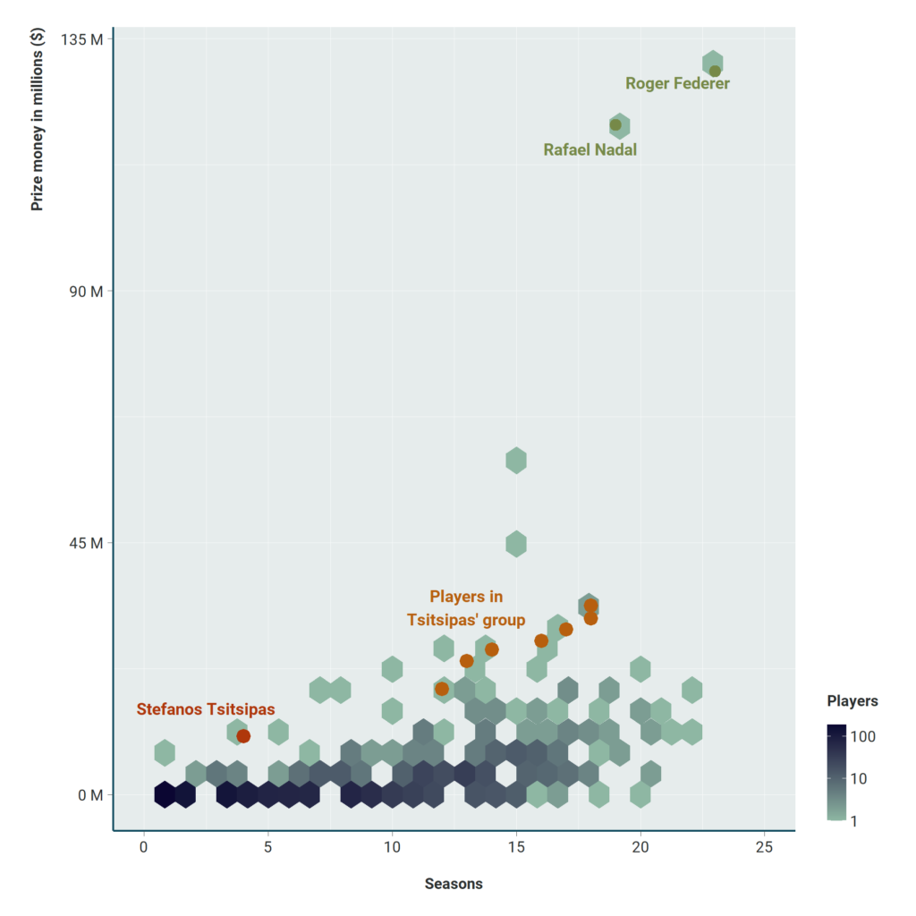
To visualize the distribution of the 1.602 players in the dataset based on – for example – their winnings in relation to seasons played, the “hexbin plot” was selected: the hexbin plot is essentially a different approach to the scatterplot, which is usually chosen to visualize the relationship between two quantitative variables. When the data is so large that the overlays do not yield a maximum of possible information, the “hexbin plot” is appropriate, as the collected data is plotted on hexagonal grids: in this case, the darker the blue color of each hexbin, the more players are concentrated on that point.
This is the result of a collaboration between iMEdD Lab and AUEB Sports Analytics Group research team aiming to promote robust quantitative analysis in sports, on both an academic and a professional level. The team works in the field of “Sports Analytics”, which includes the creation of statistical models and the production of predictions regarding sports results, draws on sports economics, and uses such tools as performance analysis, and visualization and measurement of competitive balance.
Translation: Anatoli Stavroulopoulou