
A glossary of basic terms for the beginners in data analysis and for anyone who has queries about statistical concepts that are used in the public discourse.
- categorical variable
- census
- change
- continuous variable
- correlation
- descriptive statistics
- discrete variable
- growth rate
- independent variable
- inferential statistics
- Likert scale
- mean
- median
- mode
- moving average (rolling average)
- n
- Ν
- nominal variable
- normilization
- observation
- outlier
- percentage change
- percentage point
- population
- qualitative variable
- quantitative variable
- range
- research hypothesis
- sample
- sampling
- scales
- standard deviation
- value
- variable
- variance
- z-score
Α
B
C
categorical variable
a qualitative variable whose values can be attributes with or without ranking: the categorical variables are divided into nominal and ordinal. As for the nominal variables, these are quality characteristics in well-defined, distinct, mutually exclusive and equivalent categories. The most common examples of nominal variables are nationality, marital status, religion, etc. The ordinal variable is an ordered variable (graded). For example, the degree of satisfaction with the government’s work (“not at all”, “a little”, “moderately”, “very much”, “absolutely”) is an ordinal qualitative variable.
census
a survey collecting data for all the individual units of a population. For example, during the 2019 Census of Hospitals by the Hellenic Statistical Authority (ELSTAT), data were collected from all hospitals and clinics in Greece. The most common example of a census is the population census of a country.
change
the alteration in the value or values of a variable –usually at one point in time relative to another, comparable moment. For example, according to a recent survey by ELSTAT on construction activity in Greece, in January 2021 (provisional data), 353 building permits were issued in Attica: that is, 79 more compared to January 2020, when 274 permits were issued. Most often, the change is expressed as a percentage (see percentage change). Otherwise, in case it is expressed in absolute numbers, it is only a difference, since the initial value is simply subtracted from the final one.
continuous variable
quantitative variable that can take countless values (eg 1.80, 1.805, 1.809595959 etc). In contrast, there are discrete (or discontinuous) quantitative variables that can take specific values (usually integers) –for example, the number of beds in a hospital: it can be 30, 50, 60, 100 and so on.
correlation
the term refers to a wide range of statistical relationships between variables, which can also involve dependence. It is very common for “correlation” to be used to the extent that two variables present a linear relationship –that is, whether either, as one increases, the other increases, or as one decreases, the other decreases, or as one increases, the other decreases. A common example is the correlation of the price of a product with the demand for it. There are various coefficients for calculating the correlation between two variables –the so-called “Pearson correlation coefficient“, which is named after its inspirer, the English mathematician Karl Pearson, is widely used.
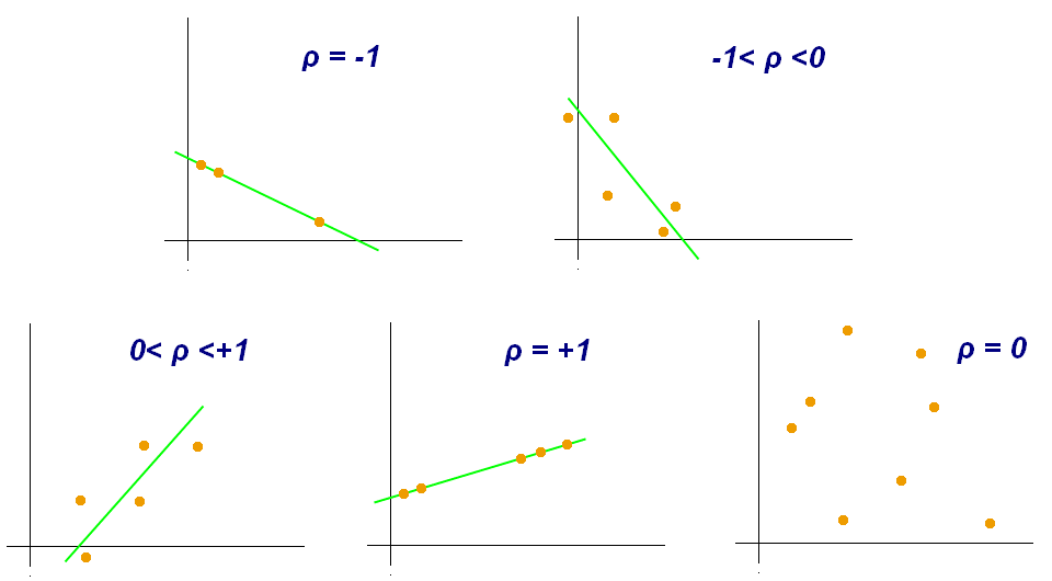
The correlation coefficient is usually denoted by the Latin letter r or the Greek ρ and can take values between -1 and 1:
-1 ≤ r ≤ 1
The closer the correlation coefficient is to 1, the stronger is the positive correlation. On the contrary, the closer the r is to -1, the stronger is the negative correlation. A correlation coefficient equal to zero (or around zero) means that there is no correlation between the two variables under study. Helpful, for understanding the correlation between two variables, is the following image from the Wikipedia.
One can calculate the correlation between two variables under study very easily, using spreadsheets and the function = CORREL().
The phrase “correlation does not imply causation” is rightly constantly repeated, meaning that the fact that one variable increases as another increases does not necessarily mean that the first increases because the second increases.
D
descriptive statistics
the branch of statistics that deals with the description of data, that is, their concise and effective presentation. For example, if when looking at a sample of 100 graduates of a university department, we report that 40 out of 100 of them, graduated with honors, then we describe what we observed. If we report that 40% of the students of the department graduate with honors, then we proceed to statistical inference (see inferential statistics). In the latter case, it is made evident how important the selection of the sample is (see sampling).
discrete variable
a quantitative variable that can take specific values. Usually, its values are integers –for instance, the number of beds in a hospital: it can be 30, 50, 60, 100 and so on. Discrete variables are also called discontinuous. On the opposite side are the continuous variables; that is the quantitative variables that can take innumerable values (eg 1.80, 1.805, 1.809595959, etc).
E
F
G
growth rate
the average percentage change of a value over time. Assuming we study linear growth, then the growth/change rate is calculated as follows:
( ( (V2 – V1) / t ) / V1 ) * 100
where V2 is the most recent value, V1 is the initial value and t is the duration.
For example, according to open data from the World Bank, the annual per capita GDP in Greece was formed, for the years from 2008 to 2015, as demonstrated in the table below (in dollars).
| 2008 | 2009 | 2010 | 2011 | 2012 | 2013 | 2014 | 2015 |
| 31997.28 | 29710.97 | 26917.76 | 25916.29 | 22242.68 | 21874.82 | 21760.98 | 18167.77 |
If we would like to calculate the annual growth rate for these seven years, we would do the following calculation:
( ( (18167.77 – 31997.28) / 7 ) / 31997.28 ) * 100 = -6,17%
Then, we could say that the annual growth rate for per capita GDP in Greece, from 2008 to 2015, was -6.17% –that is, the annual recession rate was 6.17%.
On a University of Oregon blog, we have found one of the most comprehensible explanations for the difference between rate of change and percentage change.
H
I
independent variable
a broadly used term that distinguishes variables when studying the effect of one variable (independent) on another (dependent). In general, it could be described as the variable that is not affected, but can affect another. It helps to keep in mind that, in a cause-and-effect relationship, the independent variable would represent the cause. For example, if we were to study the possible relationship between GDP per capita and life expectancy, the first would be the independent variable. If our research question was whether the level of the minimum wage affects the unemployment rate, the minimum wage would be the independent variable. In scientific, experimental research, the independent variable is managed by the researcher in order to measure its effect on the dependent variable in question. For example, the substance received by participants in a clinical trial (drug/vaccine or placebo) is the independent variable, its effect being the dependent variable. The distinction of variables into independent and dependent plays a central role in other research fields as well, such as machine learning and the creation of prediction models.
inferential statistics
also called statistical inference, is the branch of statistics that studies the characteristics and analyzes the data of a subset (see sample), in order to draw corresponding conclusions for the set (see population). Therefore, this is the statistics making inductions from sample to population. Here, it is made evident how important sampling and analysis methodology are, before drawing conclusions.
J
K
L
Likert scale
a psychometric ordinal measuring scale, originally created by the American psychologist Rensis Likert, from whom it took its name. The five-point Likert scale is widely used in social surveys. Each time we answer a “closed-ended” question by selecting “Strongly Disagree” or “Disagree” or “Neither Agree nor Disagree” or “Agree” or “Strongly Agree”, we categorize our preference based on the Likert scale.
M
mean
the average of a set of n observations –is calculated by dividing the sum of the observations by their number. It can be affected “incorrectly”; when its calculation is affected by any outliers found in the sample it may not be a realistic reflection of a situation. In this case, the average may underestimate or overestimate a situation; for this reason it is recommended to compare it with the median, which is preferred in the analysis, especially when there is a large difference between the two.
median
the average value of a set of values, arranged in ascending order. For example, assume that we have the salaries of seven employees in the following order:
700, 800, 800, 950, 1,200, 1,500, 2,000
The number 950 is the one that has on its left as many values as it has on its right (three from each side). Therefore, the median salary of these employees is 950 Euros.
If the number of observations is even, then the median is the mean of the two middle values. In the example above, while the median equals 950, the average payroll is 1,136 Euros (sum of salaries/number of employees). The reason is that the average is affected by the outliers of the sample. That is why the median is often preferred, instead of the average, in the analyses.
mode
the observation with the highest frequency, that is the value that is most often encountered in a set of values. Assume that we have the example of the monthly payroll of seven employees, which was also used above (see median):
700, 800, 800, 950, 1,200, 1,500, 2,000
Here, the mode is the 800 Euros. The median is the 950 Euros and the average is around 1,136 Euros. Analyzing the payroll of the example, one could say that, although the average salary is 950 Euros, the most common one is at 150 Euros lower. The average payroll, in fact, is set up by one relatively high-paid employee.
moving average (rolling average)
very often used in time series data in order to level short-term fluctuations (for instance, record keeping problems) and to more accurately highlight longer-term trends.
For example, in the graph above, which shows the evolution of daily COVID-19 cases in Greece over time, the line in dark blue indicates the rolling average of 7 days: it is shaped by recording, for each day, the average of daily cases, based on the data of the last seven days at a time. In this way, the values of the daily recorded cases (blue bars) –which may be affected by record keeping problems– the corresponding daily number of tests performed, etc, are leveled.
N
n
Latin letter, usually denoting the sample size. For example, when the iMEdD Lab published the geographical distribution of COVID-19 deaths in Greece in December 2020, based on a sample of 3,214 losses (a total of 3,687 until December 14), it could indicate that: n = 3,214.
Ν
Latin letter, usually denoting the size of the population –in contrast to n, which usually indicates the size of the sample. For example, when the iMEdD Lab published the geographical distribution of COVID-19 deaths in Greece in December 2020, based on a sample of 3,214 losses (a total of 3,687 as of December 14), it could indicate that: n = 3,214, N = 3,687
nominal variable
qualitative characteristics (categorical variables), placed among well-defined, distinct, mutually exclusive, and equivalent categories, which are not ranked. The most common examples of nominal variables are nationality, marital status, religion, etc.
normilization
can take many meanings in applications of statistics. In the simplest and most common case, normalization of numbers means adjusting values of different scales to a common scale in order for them to be comparable. For example, all surveys that refer to “per 100 thousand inhabitants” refer to normalized numbers. In the last year, the most common example is COVID-19 cases, the numbers of which are normalized per 100 thousand or per 1 million inhabitants –especially in analyses comparing countries or regions with different populations. If this wasn’t the case, it would be the population of the countries largely “reflected” in the case numbers.
In the above world map of cases from the beginning of the pandemic, the countries are “colored” based on the normalized cases per 100 thousand inhabitants of local population. This allows us to establish that, for example, Sweden is almost at the same place as the USA.
Ο
observation
the value that a variable takes as part of a series of data collected from selected units of the population (sample). Observations (or, in other words, statistical data) can be qualitative or numerical. In a series of data, the observations are not necessarily different. For example, if we ask ten people which party they vote for, we have ten observations. Of these, four may be common if four of the respondents respond that they vote for the same party. Or, if we ask five people in Athens from which region of Greece they are coming from, each of them can give a different answer from the 13 regions of the country. In fact, we can get answers (that is, collect observations) such as:
Central Macedonia, Central Macedonia, Attica, Crete, Thessaly, Attica
outlier
when studying only one variable/measurement, an“extreme” value (outlier) isone that lies at the edges of a statistical distribution, meaning that it is much smaller or much larger than the other values of the set under study. Thus, it can affect the mean significantly, and possibly incorrectly, which is why it is often excluded when calculating said mean. In other cases, outliers may indicate data from a different population than those in the other observations.
Ρ
percentage change
the relative difference of two numbers from one point in time to another. It is calculated by the formula:
( (V2 – V1) / V1 ) * 100,
where V2, the most recent value and V1, the initial value. For example, according to a recent survey by ELSTAT on construction activity in Greece, in January 2021 (provisional data), 353 building permits were issued in Attica, while 274 permits were issued in January 2020. Therefore, the percentage change is calculated as follows:
( (353 – 274) / 274 ) * 100 = 28,8%
This means that the issuance of building permits increased by 28.8%, compared to the same period last year.
A negative percentage change indicates a decrease. That is, if the result of the calculation was -28.8%, then we would say that there is a decrease of 28.8%.
percentage point
the numerical difference between two percentages. For example, in a poll regarding voting intention, if one party gets 30% of the answers and another party gets 24% of the answers, then the former is “ahead” by 6 percentage points (and not by “6%”).
population
a set that is examined in regards to one or more of its characteristics –usually, through the analysis of a sample, except for the case of a census. For example, if we want to examine the intention to vote in the run-up to elections, the population is the set of people eligible to vote in the upcoming elections. It is usually denoted by the Latin letter N. Population data are sometimes referred to as units.
Q
qualitative variable
the values of which are not numbers. For example, gender, religion, level of education, political affiliation, marital status are qualitative variables –they are divided into nominal and ordinal. For example, marital status is a nominal qualitative variable, while the degree of satisfaction with the government’s work (“not at all”, “a little”, “moderately”, “very much”, “absolutely”) is an ordinal qualitative variable.
quantitative variable
the values of which are numbers. Quantitative variables are divided into discrete or discontinuous and continuous variables.
R
range
the difference between the minimum and the maximum value –this is the simplest of the measures of dispersion. In the example of the payroll, the range is 1,300 Euros (2,000 – 700).
research hypothesis
a specific, clear and verifiable statement regarding the possible outcome of a research study. Defining the research hypotheses is one of the most important steps in designing a quantitative research. These hypotheses, stated in advance by the research team, often determine the design of the study. They are confirmed or refuted after statistical analysis of the data.
S
sample
a subset of a population –that is, data collected regarding the population, so that their analysis leads to safe generalizable conclusions about the set (population). The size of the statistical sample is usually denoted by the Latin letter n. For example, in a survey regarding the telecommuting of private sector employees, with the participation of 2,000 respondents, the identity of the study could indicate that n = 2,000. Then, the population, usually denoted as N, would be the total number of private employees in the country.
sampling
the method of selecting the statistical sample. Random sampling (probability samples) is suitable for empirical research, because it allows the representation of the population and the generalization of conclusions –from the sample to the population. The four types of random sampling are simple random, stratified, systematic and cluster sampling. Conversely, non-random sampling (non-probability samples) is based on criteria such as ease, availability, speed of data collection, etc, but does not allow us to generalize the results to the population.
scales
categorization of the measurement into four types: nominal or categorical, ordinal, interval and ratio scale.
standard deviation
one of the measures of dispersion (or measures of variability), with a central role in statistics. It signifies the deviation of the values of a variable from the “central” position –that is, it measures how far a set of numbers extends from the mean value of the set under study. Mathematically, it is expressed as the positive square root of the variance (see variance) and is usually denoted by the Latin letter s. In relation to the variance, the advantage of the standard deviation is that it is expressed by the same unit of measurement as the observations. For example, if we study a series of payroll data in Euros, the standard deviation will also be expressed in Euros. It helps to think that the greater the standard deviation, the greater is the dispersion of observations –that is, our data do not “cluster” enough around the average.
Τ
U
V
value
the values that a variable can take are called the variable values. For example, assume that we ask five people in Athens which region of Greece they are coming from. The variable “region” can take as a value any of the 13 regions of the country. The answers we will receive from these five people will be our observations, that is the statistical data. In a series of data, the observations are not necessarily different. In the example above, the values that the variable can take are the 13 regions of the country, but, in fact, we can get answers (that is, collect observations) such as:
Central Macedonia, Central Macedonia, Attica, Crete, Thessaly, Attica
variable
the characteristic in relation to which we examine the population under study. For example, some variables that we study on a daily basis in analyses regarding the pandemic: country, daily cases, daily deaths, intubated patients, new tests performed, daily vaccine doses, and so on.
variance
one of the measures of dispersion (or measures of variability), which plays a central role in statistics. It signifies the deviation of the values of a variable from the “central” position –that is, it measures how far a set of numbers extends from the mean value of the set under study. Mathematically, it is expressed as the mean of the squares of the deviations of the values from their mean. Thus, the disadvantage is that the variance is expressed by the square of each unit of measurement –and not by the unit of measurement in which expressed the statistical data themselves.
For example, assume that we have two sets of numbers signifying meters, as follows:
Set Α’ = 1 + 2 + 3 + 4 + 5 m.
Set Β’ = 0 + 1 + 2 + 5 + 7 m.
In both cases the set average is 3. But by calculating the variance in each set, things change.
Set Α’ – Variance:
( (1-3)2 + (2-3)2 + (3-3)2 + (4-3)2 + (5-3)2 ) / 5 =
(4 + 1 + 0 + 1 + 4) / 5 = 2 τ.μ.
Set Β’ – Variance:
( (0-3)2 + (1-3)2 + (2-3)2 + (5-3)2 + (7-3)2 ) / 5 =
(9 + 4 + 1 + 4 + 16) / 5 = 6,8 τ.μ.
In this example, the variance is expressed in square meters (sq.m.). In Set B’, the variance is greater. Thus, there is a greater dispersion of values (heterogeneity), compared to Set A’, where there is a greater “convolution” of prices around the “central” position.
W
X
Y
Z
z-score
the standardized value or z-score indicates the distance of an observation from the mean. Mathematically, it is expressed as the quotient of the following division: the difference of a value between the mean and the standard deviation –z = (x – μ) / σ, where μ is the population mean and σ is the population standard deviation). When the z-score is positive, it means that the initial value is higher than the mean –and vice versa, when the z-score is negative. Since the z-scores are expressed in standard deviation units, they are independent from the original unit of measurement. Thus, they offer the possibility of comparing prices coming from different distributions. See the z-score explained by the EuroMOMO platform and how it uses it to compare mortality in different European countries and at different times.
Analysis of Stefanos Tsitsipas’ professional trajectory
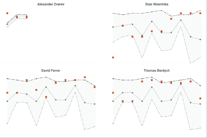
How we grouped 1,602 tennis players to find out who is more similar to Stefanos Tsitsipas and to predict the latter’s career path over the next decade, by applying simple machine learning techniques and statistical methods.
Βooks worth reading
- Darrell Huff, How to Lie with Statistics, Penguin, Λονδίνο: 1991*
- Timothy C. Urdan, Statistics in Plain English, Routledge, Νέα Υόρκη: 2016
* Or any other edition of this legendary book written by a journalist-writer in 1954 (see Darrell Huff).
Useful links
- Eurostat, Statistics Explained
- OECD, Glossary of Statistical Terms
- Royal Statistical Society, Statistics for Journalists, Science and Statistics for Journalists Workshop, RSS & NCTJ, Bloomberg, London: November 13, 2014
Thanks to Dimitris Karlis, Professor at the Department of Statistics, Athens University of Economics and Business (AUEB), for his advice and comments.
Translation: Evita Lykou

